

explicitly into a mathematical model, and this tendency is further
reinforced by the expanding computational power. However, abstraction is necessary and is done in all modeling efforts. We want to stress
here that the most important reason for using modeling approaches is
to provide mechanistic insight buried in the data, and not just to crank
machines and obtain some numbers. For this purpose, it is both
productive and necessary to perform proper abstraction and idealization as successfully used in theoretical physics [27]. A simple model
that only makes qualitative predictions but provides deep mechanistic
insight has more value than a complex model that can only “reproduce” experimental data but does not necessarily make a new set of
predictions that may be tested experimentally to improve our understanding of the system. To be fair, both detailed and simplified
approaches have their merits, and sometimes it is constructive to
combine the two strategies https://www.nature.com/articles/
s41540-020-0132-1. One may start with detailed models that can
reproduce the data, then remove model ingredients step-by-step to
identify the minimal components that are essential for recapitulating
the key dynamical features of the system.
2.3 Construct a
Mathematical Model
and Perform Analysis
With the problem identified and an appropriate modeling framework selected, one can follow some generic modeling procedures:
1. Summarize known interacting species into a regulatory network. If there are uncertain interactions, one may construct a
set of possible networks for later comparative studies. Figure 1
shows a core EMT regulatory network used in several studies
[9, 13, 28].
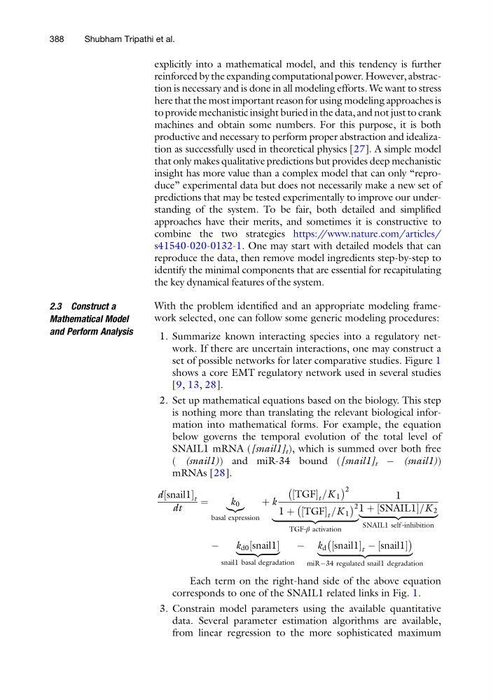
2. Set up mathematical equations based on the biology. This step
is nothing more than translating the relevant biological information into mathematical forms. For example, the equation
below governs the temporal evolution of the total level of
SNAIL1 mRNA ([snail1] t ), which is summed over both free
( (snail1)) and miR-34 bound ([snail1] t À (snail1))
mRNAs [28].
d snail1
½
t
dt
¼
k 0
|{z}
basal expression
þ k
TGF
½
t =K 1
À
Á 2
1 þ TGF
½
t =K 1
À
Á 2
|fflfflfflfflfflfflfflfflfflfflfflfflfflfflfflffl ffl{zfflfflfflfflfflfflfflfflfflfflfflfflfflfflfflffl ffl}
TGF‐β activation
1
1 þ SNAIL1
½
=K 2
|fflfflfflfflfflfflfflfflfflfflfflfflfflffl ffl{zfflfflfflfflfflfflfflfflfflfflfflfflfflffl ffl}
SNAIL1 self ‐inhibition
À
k d0 snail1
½
|fflfflfflfflfflffl ffl{zfflfflfflfflfflffl ffl}
snail1 basal degradation
À k d snail1
½
t À snail1
½
À
Á
|fflfflfflfflfflfflfflfflfflfflfflfflfflfflfflfflfflffl ffl{zfflfflfflfflfflfflfflfflfflfflfflfflfflfflfflfflfflffl ffl}
miRÀ34 regulated snail1 degradation
Each term on the right-hand side of the above equation
corresponds to one of the SNAIL1 related links in Fig. 1.
3. Constrain model parameters using the available quantitative
data. Several parameter estimation algorithms are available,
from linear regression to the more sophisticated maximum
388
Shubham Tripathi et al.
reinforced by the expanding computational power. However, abstraction is necessary and is done in all modeling efforts. We want to stress
here that the most important reason for using modeling approaches is
to provide mechanistic insight buried in the data, and not just to crank
machines and obtain some numbers. For this purpose, it is both
productive and necessary to perform proper abstraction and idealization as successfully used in theoretical physics [27]. A simple model
that only makes qualitative predictions but provides deep mechanistic
insight has more value than a complex model that can only “reproduce” experimental data but does not necessarily make a new set of
predictions that may be tested experimentally to improve our understanding of the system. To be fair, both detailed and simplified
approaches have their merits, and sometimes it is constructive to
combine the two strategies https://www.nature.com/articles/
s41540-020-0132-1. One may start with detailed models that can
reproduce the data, then remove model ingredients step-by-step to
identify the minimal components that are essential for recapitulating
the key dynamical features of the system.
2.3 Construct a
Mathematical Model
and Perform Analysis
With the problem identified and an appropriate modeling framework selected, one can follow some generic modeling procedures:
1. Summarize known interacting species into a regulatory network. If there are uncertain interactions, one may construct a
set of possible networks for later comparative studies. Figure 1
shows a core EMT regulatory network used in several studies
[9, 13, 28].
2. Set up mathematical equations based on the biology. This step
is nothing more than translating the relevant biological information into mathematical forms. For example, the equation
below governs the temporal evolution of the total level of
SNAIL1 mRNA ([snail1] t ), which is summed over both free
( (snail1)) and miR-34 bound ([snail1] t À (snail1))
mRNAs [28].
d snail1
½
t
dt
¼
k 0
|{z}
basal expression
þ k
TGF
½
t =K 1
À
Á 2
1 þ TGF
½
t =K 1
À
Á 2
|fflfflfflfflfflfflfflfflfflfflfflfflfflfflfflffl ffl{zfflfflfflfflfflfflfflfflfflfflfflfflfflfflfflffl ffl}
TGF‐β activation
1
1 þ SNAIL1
½
=K 2
|fflfflfflfflfflfflfflfflfflfflfflfflfflffl ffl{zfflfflfflfflfflfflfflfflfflfflfflfflfflffl ffl}
SNAIL1 self ‐inhibition
À
k d0 snail1
½
|fflfflfflfflfflffl ffl{zfflfflfflfflfflffl ffl}
snail1 basal degradation
À k d snail1
½
t À snail1
½
À
Á
|fflfflfflfflfflfflfflfflfflfflfflfflfflfflfflfflfflffl ffl{zfflfflfflfflfflfflfflfflfflfflfflfflfflfflfflfflfflffl ffl}
miRÀ34 regulated snail1 degradation
Each term on the right-hand side of the above equation
corresponds to one of the SNAIL1 related links in Fig. 1.
3. Constrain model parameters using the available quantitative
data. Several parameter estimation algorithms are available,
from linear regression to the more sophisticated maximum
388
Shubham Tripathi et al.