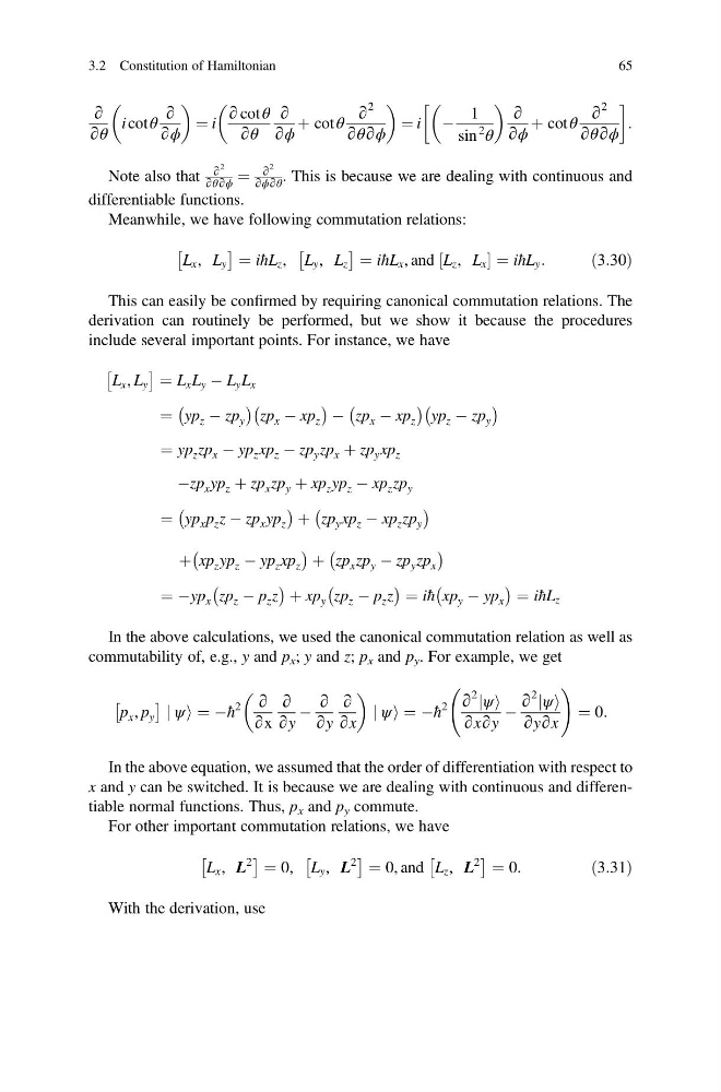
∂
∂θ
i cot θ
∂
∂ϕ
¼ i
∂ cot θ
∂θ
∂
∂ϕ
þ cot θ
∂
2
∂θ∂ϕ
¼ i À
1
sin
2
θ
∂
∂ϕ
þ cot θ
∂
2
∂θ∂ϕ
!
:
Note also that
∂
2
∂θ∂ϕ
¼
∂
2
∂ϕ∂θ
. This is because we are dealing with continuous and
differentiable functions.
Meanwhile, we have following commutation relations:
L x , L y
Â
à ¼ iħL z , L y , L z
Â
à ¼ iħL x , and L z , L x
½
Š¼iħL y :
ð3:30Þ
This can easily be confirmed by requiring canonical commutation relations. The
derivation can routinely be performed, but we show it because the procedures
include several important points. For instance, we have
L x , L y
Â
à ¼ L x L y À L y L x
¼ yp z À zp y
À
Á
zp x À xp z
À
Á À zp x À xp z
À
Á
yp z À zp y
À
Á
¼ yp z zp x À yp z xp z À zp y zp x þ zp y xp z
Àzp x yp z þ zp x zp y þ xp z yp z À xp z zp y
¼ yp x p z z À zp x yp z
À
Á þ zp y xp z À xp z zp y
À
Á
þ xp z yp z À yp z xp z
À
Á þ zp x zp y À zp y zp x
À
Á
¼ Àyp x zp z À p z z
À
Á þ xp y zp z À p z z
À
Á ¼ iħ xp y À yp x
À
Á ¼ iħL z
In the above calculations, we used the canonical commutation relation as well as
commutability of, e.g., y and p x ; y and z; p x and p y . For example, we get
p x , p y
Â
à j ψi ¼ Àħ
2 ∂
∂x
∂
∂y
À
∂
∂y
∂
∂x
j ψi ¼ Àħ
2 ∂
2 jψi
∂x∂y
À
∂
2 jψi
∂y∂x
!
¼ 0:
In the above equation, we assumed that the order of differentiation with respect to
x and y can be switched. It is because we are dealing with continuous and differentiable normal functions. Thus, p x and p y commute.
For other important commutation relations, we have
L x , L
2
Â
à ¼ 0, L y , L
2
Â
à ¼ 0, and L z , L
2
Â
à ¼ 0:
ð3:31Þ
With the derivation, use
3.2 Constitution of Hamiltonian
65