

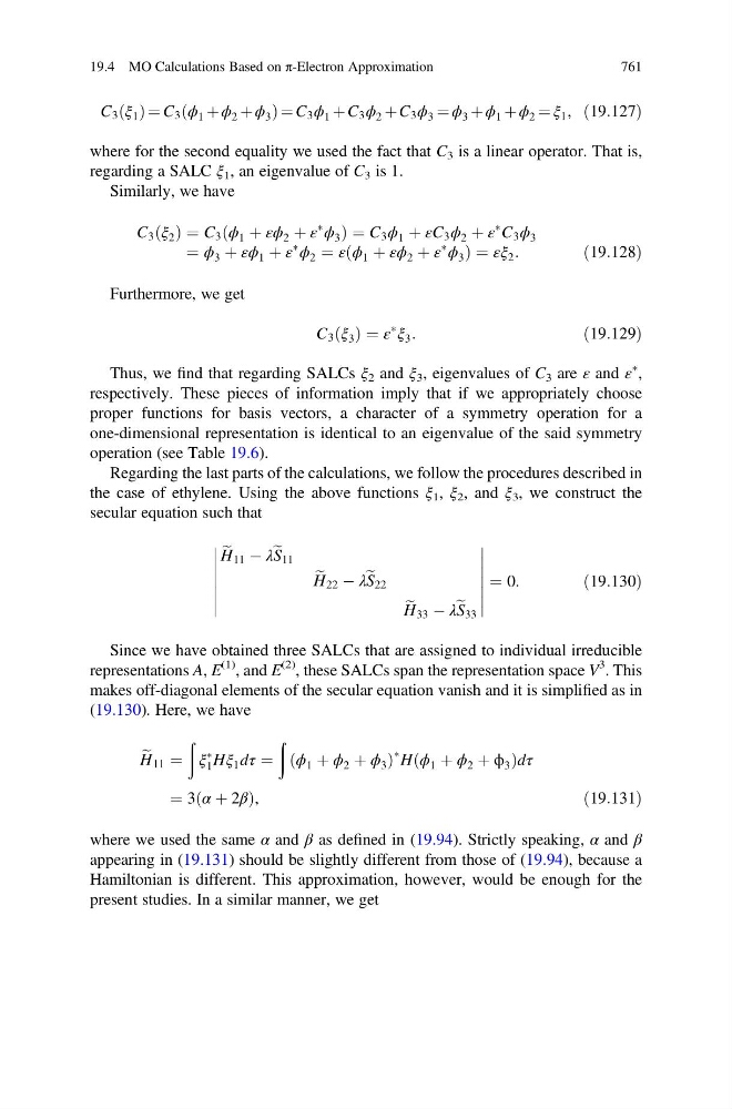
C 3 ξ 1
ð Þ¼C 3 ϕ 1 þ ϕ 2 þ ϕ 3
ð
Þ ¼ C 3 ϕ 1 þ C 3 ϕ 2 þ C 3 ϕ 3 ¼ ϕ 3 þ ϕ 1 þ ϕ 2 ¼ ξ 1 , ð19:127Þ
where for the second equality we used the fact that C 3 is a linear operator. That is,
regarding a SALC ξ 1 , an eigenvalue of C 3 is 1.
Similarly, we have
C 3 ξ 2
ð Þ ¼ C 3 ϕ 1 þ εϕ 2 þ ε
Ã
ϕ 3
ð
Þ ¼ C 3 ϕ 1 þ εC 3 ϕ 2 þ ε
à C 3 ϕ 3
¼ ϕ 3 þ εϕ 1 þ ε
Ã
ϕ 2 ¼ ε ϕ 1 þ εϕ 2 þ ε
Ã
ϕ 3
ð
Þ ¼ εξ 2 :
ð19:128Þ
Furthermore, we get
C 3 ξ 3
ð Þ ¼ ε
Ã
ξ 3 :
ð19:129Þ
Thus, we find that regarding SALCs ξ 2 and ξ 3 , eigenvalues of C 3 are ε and ε
à ,
respectively. These pieces of information imply that if we appropriately choose
proper functions for basis vectors, a character of a symmetry operation for a
one-dimensional representation is identical to an eigenvalue of the said symmetry
operation (see Table 19.6).
Regarding the last parts of the calculations, we follow the procedures described in
the case of ethylene. Using the above functions ξ 1 , ξ 2 , and ξ 3 , we construct the
secular equation such that
e
H 11 À λ e S 11
e
H 22 À λ e S 22
e
H 33 À λ e S 33
¼ 0:
ð19:130Þ
Since we have obtained three SALCs that are assigned to individual irreducible
representations A, E
(1) , and E
(2) , these SALCs span the representation space V
3 . This
makes off-diagonal elements of the secular equation vanish and it is simplified as in
(19.130). Here, we have
e
H 11 ¼
ð
ξ
Ã
1 Hξ 1 dτ ¼
ð
ϕ 1 þ ϕ 2 þ ϕ 3
ð
Þ
à H ϕ 1 þ ϕ 2 þ ϕ 3
ð
Þ dτ
¼ 3 α þ 2β
ð
Þ,
ð19:131Þ
where we used the same α and β as defined in (19.94). Strictly speaking, α and β
appearing in (19.131) should be slightly different from those of (19.94), because a
Hamiltonian is different. This approximation, however, would be enough for the
present studies. In a similar manner, we get
19.4 MO Calculations Based on π-Electron Approximation
761