

e
P
T ¼ R 1 R
1
ð Þ
2 R
2
ð Þ
3 Á Á ÁR
nÀ3
ð
Þ
nÀ2 R
nÀ2
ð
Þ
nÀ1
h
i T ¼ R
nÀ2
ð
Þ
nÀ1
h
i T
R
nÀ3
ð
Þ
nÀ2
h
i T Á Á Á R
1
ð Þ
2
h
i T
R 1
½
T
¼ R
nÀ2
ð
Þ
nÀ1
h
i À1
R
nÀ3
ð
Þ
nÀ2
h
i À1 Á Á Á R
1
ð Þ
2
h
i À1
R 1
À1
Â
Ã
¼ R 1 R
1
ð Þ
2 R
2
ð Þ
3 Á Á ÁR
nÀ3
ð
Þ
nÀ2 R
nÀ2
ð
Þ
nÀ1
h
i À1 ¼ e
P
À1
:
ð17:99Þ
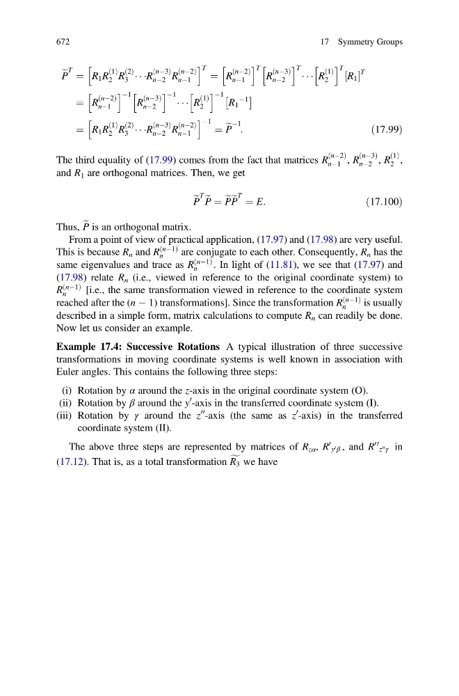
The third equality of (17.99) comes from the fact that matrices R
nÀ2
ð
Þ
nÀ1 , R
nÀ3
ð
Þ
nÀ2 , R
1
ð Þ
2 ,
and R 1 are orthogonal matrices. Then, we get
e
P
T
e
P ¼ e
P e
P
T ¼ E:
ð17:100Þ
Thus, e
P is an orthogonal matrix.
From a point of view of practical application, (17.97) and (17.98) are very useful.
This is because R n and R
nÀ1
ð
Þ
n
are conjugate to each other. Consequently, R n has the
same eigenvalues and trace as R
nÀ1
ð
Þ
n
. In light of (11.81), we see that (17.97) and
(17.98) relate R n (i.e., viewed in reference to the original coordinate system) to
R
nÀ1
ð
Þ
n
[i.e., the same transformation viewed in reference to the coordinate system
reached after the (n À 1) transformations]. Since the transformation R
nÀ1
ð
Þ
n
is usually
described in a simple form, matrix calculations to compute R n can readily be done.
Now let us consider an example.
Example 17.4: Successive Rotations A typical illustration of three successive
transformations in moving coordinate systems is well known in association with
Euler angles. This contains the following three steps:
(i) Rotation by α around the z-axis in the original coordinate system (O).
(ii) Rotation by β around the y
0 -axis in the transferred coordinate system (I).
(iii) Rotation by γ around the z
00
-axis (the same as z
0 -axis) in the transferred
coordinate system (II).
The above three steps are represented by matrices of R zα , R
0
y 0 β , and R
00
z 00 γ in
(17.12). That is, as a total transformation f
R 3 we have
672
17 Symmetry Groups
P
T ¼ R 1 R
1
ð Þ
2 R
2
ð Þ
3 Á Á ÁR
nÀ3
ð
Þ
nÀ2 R
nÀ2
ð
Þ
nÀ1
h
i T ¼ R
nÀ2
ð
Þ
nÀ1
h
i T
R
nÀ3
ð
Þ
nÀ2
h
i T Á Á Á R
1
ð Þ
2
h
i T
R 1
½
T
¼ R
nÀ2
ð
Þ
nÀ1
h
i À1
R
nÀ3
ð
Þ
nÀ2
h
i À1 Á Á Á R
1
ð Þ
2
h
i À1
R 1
À1
Â
Ã
¼ R 1 R
1
ð Þ
2 R
2
ð Þ
3 Á Á ÁR
nÀ3
ð
Þ
nÀ2 R
nÀ2
ð
Þ
nÀ1
h
i À1 ¼ e
P
À1
:
ð17:99Þ
The third equality of (17.99) comes from the fact that matrices R
nÀ2
ð
Þ
nÀ1 , R
nÀ3
ð
Þ
nÀ2 , R
1
ð Þ
2 ,
and R 1 are orthogonal matrices. Then, we get
e
P
T
e
P ¼ e
P e
P
T ¼ E:
ð17:100Þ
Thus, e
P is an orthogonal matrix.
From a point of view of practical application, (17.97) and (17.98) are very useful.
This is because R n and R
nÀ1
ð
Þ
n
are conjugate to each other. Consequently, R n has the
same eigenvalues and trace as R
nÀ1
ð
Þ
n
. In light of (11.81), we see that (17.97) and
(17.98) relate R n (i.e., viewed in reference to the original coordinate system) to
R
nÀ1
ð
Þ
n
[i.e., the same transformation viewed in reference to the coordinate system
reached after the (n À 1) transformations]. Since the transformation R
nÀ1
ð
Þ
n
is usually
described in a simple form, matrix calculations to compute R n can readily be done.
Now let us consider an example.
Example 17.4: Successive Rotations A typical illustration of three successive
transformations in moving coordinate systems is well known in association with
Euler angles. This contains the following three steps:
(i) Rotation by α around the z-axis in the original coordinate system (O).
(ii) Rotation by β around the y
0 -axis in the transferred coordinate system (I).
(iii) Rotation by γ around the z
00
-axis (the same as z
0 -axis) in the transferred
coordinate system (II).
The above three steps are represented by matrices of R zα , R
0
y 0 β , and R
00
z 00 γ in
(17.12). That is, as a total transformation f
R 3 we have
672
17 Symmetry Groups