

Z 1
À1
f
ψ m ξ
ð Þ
à f
ψ n ξ
ð Þdξ ¼ δ mn :
ð2:104Þ
Placing (2.98) back into the function form ψ n (q), we have
ψ n q
ð Þ ¼
ffiffiffi
β
p f
ψ n βq
ð Þ:
ð2:105Þ
Using (2.101) and explicitly rewriting (2.105), we get
ψ n q
ð Þ ¼
mω
ħ
1=4
ffiffiffiffiffiffiffiffiffiffiffiffiffiffiffiffi
1
π 1=2 2
n n!
r
H n
ffiffiffiffiffiffiffi
mω
ħ
r
q
e
À
mω
2ħ q
2
n ¼ 0, 1, 2, Á Á Á
ð
Þ :
ð2:106Þ
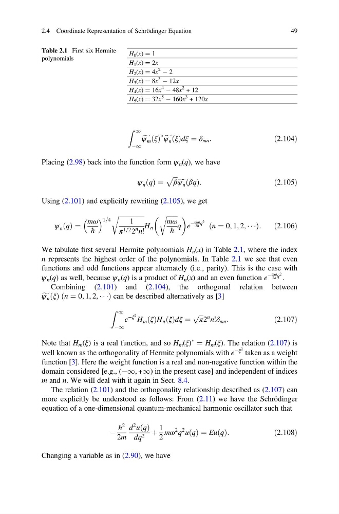
We tabulate first several Hermite polynomials H n (x) in Table 2.1, where the index
n represents the highest order of the polynomials. In Table 2.1 we see that even
functions and odd functions appear alternately (i.e., parity). This is the case with
ψ n (q) as well, because ψ n (q) is a product of H n (x) and an even function e
À
mω
2ħ q
2 .
Combining (2.101) and (2.104), the orthogonal relation between
f
ψ n ξ
ð Þ n ¼ 0, 1, 2, Á Á Á
ð
Þcan be described alternatively as [3]
Z 1
À1
e
Àξ
2
H m ξ
ð ÞH n ξ
ð Þdξ ¼
ffiffiffi
π
p
2
n n!δ mn :
ð2:107Þ
Note that H m (ξ) is a real function, and so H m (ξ)
Ã
¼ H m (ξ). The relation (2.107) is
well known as the orthogonality of Hermite polynomials with e
Àξ
2 taken as a weight
function [3]. Here the weight function is a real and non-negative function within the
domain considered [e.g., (À1, +1) in the present case] and independent of indices
m and n. We will deal with it again in Sect. 8.4.
The relation (2.101) and the orthogonality relationship described as (2.107) can
more explicitly be understood as follows: From (2.11) we have the Schrödinger
equation of a one-dimensional quantum-mechanical harmonic oscillator such that
À
ħ
2
2m
d
2 u q
ð Þ
dq 2 þ
1
2
mω
2 q
2 u q
ð Þ ¼ Eu q
ð Þ:
ð2:108Þ
Changing a variable as in (2.90), we have
Table 2.1 First six Hermite
polynomials
H 0 (x) ¼ 1
H 1 (x) ¼ 2x
H 2 (x) ¼ 4x
2 À 2
H 3 (x) ¼ 8x
3 À 12x
H 4 (x) ¼ 16x
4 À 48x
2 + 12
H 5 (x) ¼ 32x
5 À 160x
3 + 120x
2.4 Coordinate Representation of Schrödinger Equation
49
À1
f
ψ m ξ
ð Þ
à f
ψ n ξ
ð Þdξ ¼ δ mn :
ð2:104Þ
Placing (2.98) back into the function form ψ n (q), we have
ψ n q
ð Þ ¼
ffiffiffi
β
p f
ψ n βq
ð Þ:
ð2:105Þ
Using (2.101) and explicitly rewriting (2.105), we get
ψ n q
ð Þ ¼
mω
ħ
1=4
ffiffiffiffiffiffiffiffiffiffiffiffiffiffiffiffi
1
π 1=2 2
n n!
r
H n
ffiffiffiffiffiffiffi
mω
ħ
r
q
e
À
mω
2ħ q
2
n ¼ 0, 1, 2, Á Á Á
ð
Þ :
ð2:106Þ
We tabulate first several Hermite polynomials H n (x) in Table 2.1, where the index
n represents the highest order of the polynomials. In Table 2.1 we see that even
functions and odd functions appear alternately (i.e., parity). This is the case with
ψ n (q) as well, because ψ n (q) is a product of H n (x) and an even function e
À
mω
2ħ q
2 .
Combining (2.101) and (2.104), the orthogonal relation between
f
ψ n ξ
ð Þ n ¼ 0, 1, 2, Á Á Á
ð
Þcan be described alternatively as [3]
Z 1
À1
e
Àξ
2
H m ξ
ð ÞH n ξ
ð Þdξ ¼
ffiffiffi
π
p
2
n n!δ mn :
ð2:107Þ
Note that H m (ξ) is a real function, and so H m (ξ)
Ã
¼ H m (ξ). The relation (2.107) is
well known as the orthogonality of Hermite polynomials with e
Àξ
2 taken as a weight
function [3]. Here the weight function is a real and non-negative function within the
domain considered [e.g., (À1, +1) in the present case] and independent of indices
m and n. We will deal with it again in Sect. 8.4.
The relation (2.101) and the orthogonality relationship described as (2.107) can
more explicitly be understood as follows: From (2.11) we have the Schrödinger
equation of a one-dimensional quantum-mechanical harmonic oscillator such that
À
ħ
2
2m
d
2 u q
ð Þ
dq 2 þ
1
2
mω
2 q
2 u q
ð Þ ¼ Eu q
ð Þ:
ð2:108Þ
Changing a variable as in (2.90), we have
Table 2.1 First six Hermite
polynomials
H 0 (x) ¼ 1
H 1 (x) ¼ 2x
H 2 (x) ¼ 4x
2 À 2
H 3 (x) ¼ 8x
3 À 12x
H 4 (x) ¼ 16x
4 À 48x
2 + 12
H 5 (x) ¼ 32x
5 À 160x
3 + 120x
2.4 Coordinate Representation of Schrödinger Equation
49