

x t
ð Þ ¼ c þ σ
ð
Þe
t
À c,
y t
ð Þ ¼ c þ σ
ð
Þte
t
þ d À c þ τ
ð
Þ e
t
þ c À d:
ð15:138Þ
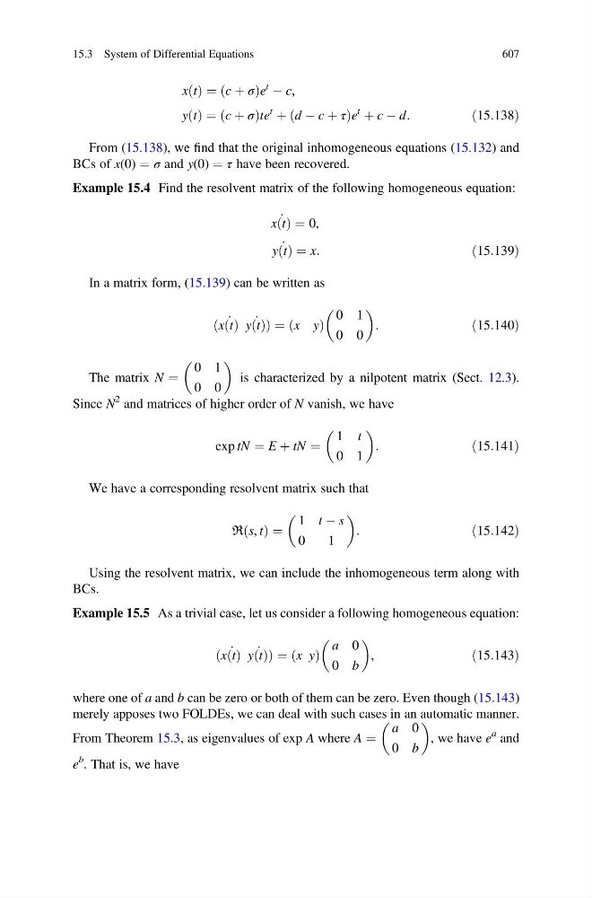
From (15.138), we find that the original inhomogeneous equations (15.132) and
BCs of x(0) ¼ σ and y(0) ¼ τ have been recovered.
Example 15.4 Find the resolvent matrix of the following homogeneous equation:
_
x t
ð Þ ¼ 0,
_
y t
ð Þ ¼ x:
ð15:139Þ
In a matrix form, (15.139) can be written as
ð _
x t
ð Þ _
y t
ð ÞÞ ¼ x y
ð
Þ
0 1
0 0
:
ð15:140Þ
The matrix N ¼
0 1
0 0
is characterized by a nilpotent matrix (Sect. 12.3).
Since N
2 and matrices of higher order of N vanish, we have
exp tN ¼ E þ tN ¼
1 t
0 1
:
ð15:141Þ
We have a corresponding resolvent matrix such that
R s, t
ð Þ ¼
1 t À s
0
1
:
ð15:142Þ
Using the resolvent matrix, we can include the inhomogeneous term along with
BCs.
Example 15.5 As a trivial case, let us consider a following homogeneous equation:
ð _
x t
ð Þ _
y t
ð ÞÞ ¼ x y
ð Þ
a 0
0 b
,
ð15:143Þ
where one of a and b can be zero or both of them can be zero. Even though (15.143)
merely apposes two FOLDEs, we can deal with such cases in an automatic manner.
From Theorem 15.3, as eigenvalues of exp A where A ¼
a 0
0 b
, we have e
a and
e
b . That is, we have
15.3 System of Differential Equations
607
ð Þ ¼ c þ σ
ð
Þe
t
À c,
y t
ð Þ ¼ c þ σ
ð
Þte
t
þ d À c þ τ
ð
Þ e
t
þ c À d:
ð15:138Þ
From (15.138), we find that the original inhomogeneous equations (15.132) and
BCs of x(0) ¼ σ and y(0) ¼ τ have been recovered.
Example 15.4 Find the resolvent matrix of the following homogeneous equation:
_
x t
ð Þ ¼ 0,
_
y t
ð Þ ¼ x:
ð15:139Þ
In a matrix form, (15.139) can be written as
ð _
x t
ð Þ _
y t
ð ÞÞ ¼ x y
ð
Þ
0 1
0 0
:
ð15:140Þ
The matrix N ¼
0 1
0 0
is characterized by a nilpotent matrix (Sect. 12.3).
Since N
2 and matrices of higher order of N vanish, we have
exp tN ¼ E þ tN ¼
1 t
0 1
:
ð15:141Þ
We have a corresponding resolvent matrix such that
R s, t
ð Þ ¼
1 t À s
0
1
:
ð15:142Þ
Using the resolvent matrix, we can include the inhomogeneous term along with
BCs.
Example 15.5 As a trivial case, let us consider a following homogeneous equation:
ð _
x t
ð Þ _
y t
ð ÞÞ ¼ x y
ð Þ
a 0
0 b
,
ð15:143Þ
where one of a and b can be zero or both of them can be zero. Even though (15.143)
merely apposes two FOLDEs, we can deal with such cases in an automatic manner.
From Theorem 15.3, as eigenvalues of exp A where A ¼
a 0
0 b
, we have e
a and
e
b . That is, we have
15.3 System of Differential Equations
607