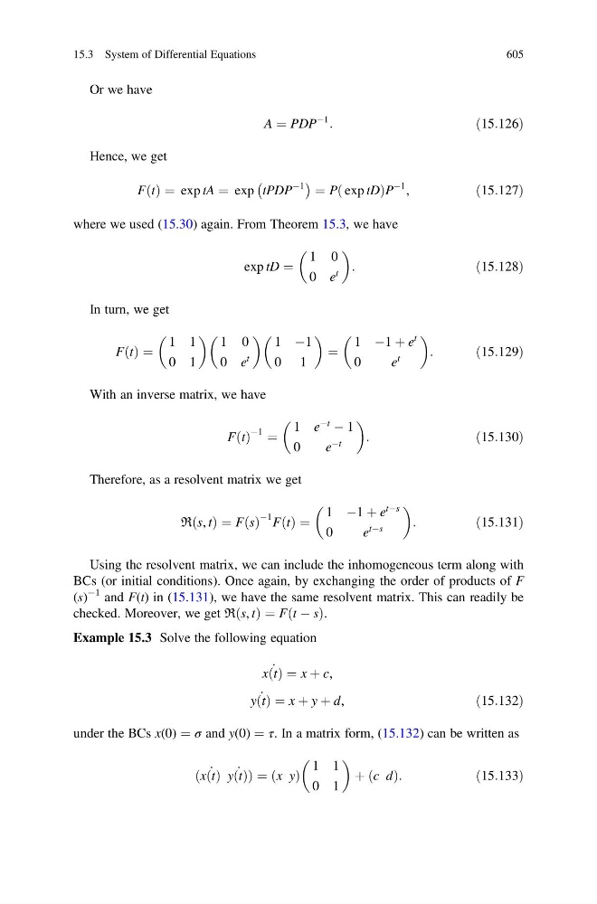
Or we have
A ¼ PDP
À1
:
ð15:126Þ
Hence, we get
F t
ð Þ ¼ exp tA ¼ exp tPDP
À1
À
Á ¼ P exp tD
ð
ÞP
À1 ,
ð15:127Þ
where we used (15.30) again. From Theorem 15.3, we have
exp tD ¼
1 0
0 e
t
:
ð15:128Þ
In turn, we get
F t
ð Þ ¼
1 1
0 1
1 0
0 e
t
1 À1
0 1
¼
1 À1 þ e
t
0
e
t
:
ð15:129Þ
With an inverse matrix, we have
F t
ð Þ
À1 ¼
1 e
Àt
À 1
0
e
Àt
:
ð15:130Þ
Therefore, as a resolvent matrix we get
R s, t
ð Þ ¼ F s
ð Þ
À1 F t
ð Þ ¼
1 À1 þ e
tÀs
0
e
tÀs
:
ð15:131Þ
Using the resolvent matrix, we can include the inhomogeneous term along with
BCs (or initial conditions). Once again, by exchanging the order of products of F
(s)
À1 and F(t) in (15.131), we have the same resolvent matrix. This can readily be
checked. Moreover, we get R s, t
ð Þ ¼ F t À s
ð
Þ.
Example 15.3 Solve the following equation
_
x t
ð Þ ¼ x þ c,
_
y t
ð Þ ¼ x þ y þ d,
ð15:132Þ
under the BCs x(0) ¼ σ and y(0) ¼ τ. In a matrix form, (15.132) can be written as
ð _
x t
ð Þ _
y t
ð ÞÞ ¼ x y
ð Þ
1 1
0 1
þ c d
ð Þ:
ð15:133Þ
15.3 System of Differential Equations
605