ð _
x t
ð Þ _
y t
ð ÞÞ ¼ x t
ð Þ y t
ð Þ
ð
Þ
a c
b d
þ p q
ð
Þ:
ð15:77Þ
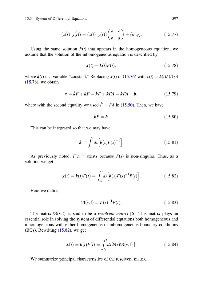
Using the same solution F(t) that appears in the homogeneous equation, we
assume that the solution of the inhomogeneous equation is described by
x t
ð Þ ¼ k t
ð ÞF t
ð Þ,
ð15:78Þ
where k(t) is a variable “constant.” Replacing x(t) in (15.76) with x(t) ¼ k(t)F(t) of
(15.78), we obtain
_
x ¼ _
kF þ k _
F ¼ _
kF þ kFA ¼ kFA þ b,
ð15:79Þ
where with the second equality we used _
F ¼ FA in (15.50). Then, we have
_
kF ¼ b:
ð15:80Þ
This can be integrated so that we may have
k ¼
Z t
ds b s
ð ÞF s
ð Þ
À1
h
i
:
ð15:81Þ
As previously noted, F(s)
À1 exists because F(s) is non-singular. Thus, as a
solution we get
x t
ð Þ ¼ k t
ð ÞF t
ð Þ ¼
Z t
t 0
ds b s
ð ÞF s
ð Þ
À1 F t
ð Þ
h
i
:
ð15:82Þ
Here we define
R s, t
ð Þ F s
ð Þ
À1 F t
ð Þ:
ð15:83Þ
The matrix R s, t
ð Þ is said to be a resolvent matrix [6]. This matrix plays an
essential role in solving the system of differential equations both homogeneous and
inhomogeneous with either homogeneous or inhomogeneous boundary conditions
(BCs). Rewriting (15.82), we get
x t
ð Þ ¼ k t
ð ÞF t
ð Þ ¼
Z t
t 0
ds b s
ð Þℜ s, t
ð Þ
½
Š :
ð15:84Þ
We summarize principal characteristics of the resolvent matrix.
15.3 System of Differential Equations
597