

_
x t
ð Þ þ p t
ð Þx ¼ q t
ð Þ:
ð15:60Þ
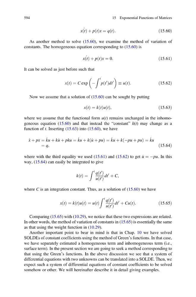
As another method to solve (15.60), we examine the method of variation of
constants. The homogeneous equation corresponding to (15.60) is
_
x t
ð Þ þ p t
ð Þx ¼ 0:
ð15:61Þ
It can be solved as just before such that
x t
ð Þ ¼ C exp À
Z t
p t
0
ð Þdt
0
u t
ð Þ:
ð15:62Þ
Now we assume that a solution of (15.60) can be sought by putting
x t
ð Þ ¼ k t
ð Þu t
ð Þ,
ð15:63Þ
where we assume that the functional form u(t) remains unchanged in the inhomogeneous equation (15.60) and that instead the “constant” k(t) may change as a
function of t. Inserting (15.63) into (15.60), we have
_
x þ px ¼ _
ku þ k _
u þ pku ¼ _
ku þ k _
u þ pu
ð
Þ¼ _
ku þ k Àpu þ pu
ð
Þ¼ _
ku
¼ q,
ð15:64Þ
where with the third equality we used (15.61) and (15.62) to get _
u ¼ Àpu. In this
way, (15.64) can easily be integrated to give
k t
ð Þ ¼
Z t q t
0
ð Þ
u t 0
ð Þ
dt
0
þ C,
where C is an integration constant. Thus, as a solution of (15.60) we have
x t
ð Þ ¼ k t
ð Þu t
ð Þ ¼ u t
ð Þ
Z t q t
0
ð Þ
u t 0
ð Þ
dt
0
þ Cu t
ð Þ:
ð15:65Þ
Comparing (15.65) with (10.29), we notice that these two expressions are related.
In other words, the method of variation of constants in (15.65) is essentially the same
as that using the weight function in (10.29).
Another important point to bear in mind is that in Chap. 10 we have solved
SOLDEs of constant coefficients using the method of Green’s functions. In that case,
we have separately estimated a homogeneous term and inhomogeneous term (i.e.,
surface term). In the present section we are going to seek a method corresponding to
that using the Green’s functions. In the above discussion we see that a system of
differential equations with two unknowns can be translated into a SOLDE. Then, we
expect such a system of differential equations of constant coefficients to be solved
somehow or other. We will hereinafter describe it in detail giving examples.
594
15 Exponential Functions of Matrices
x t
ð Þ þ p t
ð Þx ¼ q t
ð Þ:
ð15:60Þ
As another method to solve (15.60), we examine the method of variation of
constants. The homogeneous equation corresponding to (15.60) is
_
x t
ð Þ þ p t
ð Þx ¼ 0:
ð15:61Þ
It can be solved as just before such that
x t
ð Þ ¼ C exp À
Z t
p t
0
ð Þdt
0
u t
ð Þ:
ð15:62Þ
Now we assume that a solution of (15.60) can be sought by putting
x t
ð Þ ¼ k t
ð Þu t
ð Þ,
ð15:63Þ
where we assume that the functional form u(t) remains unchanged in the inhomogeneous equation (15.60) and that instead the “constant” k(t) may change as a
function of t. Inserting (15.63) into (15.60), we have
_
x þ px ¼ _
ku þ k _
u þ pku ¼ _
ku þ k _
u þ pu
ð
Þ¼ _
ku þ k Àpu þ pu
ð
Þ¼ _
ku
¼ q,
ð15:64Þ
where with the third equality we used (15.61) and (15.62) to get _
u ¼ Àpu. In this
way, (15.64) can easily be integrated to give
k t
ð Þ ¼
Z t q t
0
ð Þ
u t 0
ð Þ
dt
0
þ C,
where C is an integration constant. Thus, as a solution of (15.60) we have
x t
ð Þ ¼ k t
ð Þu t
ð Þ ¼ u t
ð Þ
Z t q t
0
ð Þ
u t 0
ð Þ
dt
0
þ Cu t
ð Þ:
ð15:65Þ
Comparing (15.65) with (10.29), we notice that these two expressions are related.
In other words, the method of variation of constants in (15.65) is essentially the same
as that using the weight function in (10.29).
Another important point to bear in mind is that in Chap. 10 we have solved
SOLDEs of constant coefficients using the method of Green’s functions. In that case,
we have separately estimated a homogeneous term and inhomogeneous term (i.e.,
surface term). In the present section we are going to seek a method corresponding to
that using the Green’s functions. In the above discussion we see that a system of
differential equations with two unknowns can be translated into a SOLDE. Then, we
expect such a system of differential equations of constant coefficients to be solved
somehow or other. We will hereinafter describe it in detail giving examples.
594
15 Exponential Functions of Matrices