_
y t
ð Þ ¼ c t
ð Þx t
ð Þ þ d t
ð Þy t
ð Þ,
ð15:55Þ
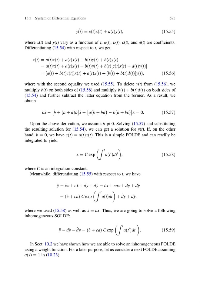
where x(t) and y(t) vary as a function of t; a(t), b(t), c(t), and d(t) are coefficients.
Differentiating (15.54) with respect to t, we get
€
x t
ð Þ ¼ _
a t
ð Þx t
ð Þ þ a t
ð Þ _
x t
ð Þ þ _
b t
ð Þy t
ð Þ þ b t
ð Þ _
y t
ð Þ
¼ _
a t
ð Þx t
ð Þ þ a t
ð Þ _
x t
ð Þ þ _
b t
ð Þy t
ð Þ þ b t
ð Þ c t
ð Þx t
ð Þ þ d t
ð Þy t
ð Þ
½
Š
¼ ½ _
a t
ð Þ þ b t
ð Þc t
ð ފx t
ð Þ þ a t
ð Þ _
x t
ð Þ þ ½ _
b t
ð Þ þ b t
ð Þd t
ð ފy t
ð Þ,
ð15:56Þ
where with the second equality we used (15.55). To delete y(t) from (15.56), we
multiply b(t) on both sides of (15.56) and multiply _
b t
ð Þ þ b t
ð Þd t
ð Þ on both sides of
(15.54) and further subtract the latter equation from the former. As a result, we
obtain
b€ x À _
b þ a þ d
ð
Þb
Â
à _
x þ a _
b þ bd
À
Á À b _
a þ bc
ð
Þ
Â
Ã
x ¼ 0:
ð15:57Þ
Upon the above derivation, we assume b 6 ¼ 0. Solving (15.57) and substituting
the resulting solution for (15.54), we can get a solution for y(t). If, on the other
hand, b ¼ 0, we have _
x t
ð Þ ¼ a t
ð Þx t
ð Þ. This is a simple FOLDE and can readily be
integrated to yield
x ¼ C exp
Z t
a t
0
ð Þdt
0
,
ð15:58Þ
where C is an integration constant.
Meanwhile, differentiating (15.55) with respect to t, we have
€ y ¼ _
cx þ c_ x þ _
dy þ d _
y ¼ _
cx þ cax þ _
dy þ d _
y
¼ _
c þ ca
ð
ÞC exp
Z t
a t
ð Þdt
þ _
dy þ d _
y,
where we used (15.58) as well as _
x ¼ ax. Thus, we are going to solve a following
inhomogeneous SOLDE:
€ y À d _
y À _
dy ¼ _
c þ ca
ð
ÞC exp
Z t
a t
0
ð Þdt
0
:
ð15:59Þ
In Sect. 10.2 we have shown how we are able to solve an inhomogeneous FOLDE
using a weight function. For a later purpose, let us consider a next FOLDE assuming
a(x) 1 in (10.23):
15.3 System of Differential Equations
593