

a
{
j ψ nÀ1 i ¼
ffiffi ffi
n
p j ψ n i:
ð2:61Þ
Or replacing n with n + 1, we get
a
{
j ψ n i ¼
ffiffiffiffiffiffiffiffiffiffiffi
n þ 1
p
j ψ nþ1
:
ð2:62Þ
As implied in (2.55) and (2.62), we find that operating a on jψ n i lowers an energy
level by one and that operating a
{ on jψ n i raises an energy level by one. For this
reason, a and a
{ are said to be an annihilation operator and creation operator,
respectively.
2.3 Matrix Representation of Physical Quantities
Equations (2.55) and (2.62) clearly represent the relationship between an operator
and eigenfunction (or eigenvector). The relationship is characterized by
Matrix
ð
ÞÂ Vector
ð
Þ¼ Vector
ð
Þ:
ð2:63Þ
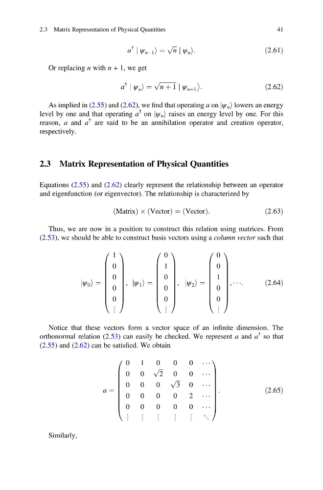
Thus, we are now in a position to construct this relation using matrices. From
(2.53), we should be able to construct basis vectors using a column vector such that
ψ 0
j i ¼
1
0
0
0
0
⋮
0
B
B
B
B
B
B
B
B
@
1
C
C
C
C
C
C
C
C
A
, ψ 1
j i ¼
0
1
0
0
0
⋮
0
B
B
B
B
B
B
B
B
@
1
C
C
C
C
C
C
C
C
A
, ψ 2
j i ¼
0
0
1
0
0
⋮
0
B
B
B
B
B
B
B
B
@
1
C
C
C
C
C
C
C
C
A
, Á Á Á:
ð2:64Þ
Notice that these vectors form a vector space of an infinite dimension. The
orthonormal relation (2.53) can easily be checked. We represent a and a
{ so that
(2.55) and (2.62) can be satisfied. We obtain
a ¼
0 1
0
0
0 Á Á Á
0 0
ffiffi ffi
2
p
0
0 Á Á Á
0 0
0
ffiffi ffi
3
p
0 Á Á Á
0 0
0
0
2 Á Á Á
0 0
0
0
0 Á Á Á
⋮ ⋮ ⋮ ⋮ ⋮ ⋱
0
B
B
B
B
B
B
B
B
@
1
C
C
C
C
C
C
C
C
A
:
ð2:65Þ
Similarly,
2.3 Matrix Representation of Physical Quantities
41
{
j ψ nÀ1 i ¼
ffiffi ffi
n
p j ψ n i:
ð2:61Þ
Or replacing n with n + 1, we get
a
{
j ψ n i ¼
ffiffiffiffiffiffiffiffiffiffiffi
n þ 1
p
j ψ nþ1
:
ð2:62Þ
As implied in (2.55) and (2.62), we find that operating a on jψ n i lowers an energy
level by one and that operating a
{ on jψ n i raises an energy level by one. For this
reason, a and a
{ are said to be an annihilation operator and creation operator,
respectively.
2.3 Matrix Representation of Physical Quantities
Equations (2.55) and (2.62) clearly represent the relationship between an operator
and eigenfunction (or eigenvector). The relationship is characterized by
Matrix
ð
ÞÂ Vector
ð
Þ¼ Vector
ð
Þ:
ð2:63Þ
Thus, we are now in a position to construct this relation using matrices. From
(2.53), we should be able to construct basis vectors using a column vector such that
ψ 0
j i ¼
1
0
0
0
0
⋮
0
B
B
B
B
B
B
B
B
@
1
C
C
C
C
C
C
C
C
A
, ψ 1
j i ¼
0
1
0
0
0
⋮
0
B
B
B
B
B
B
B
B
@
1
C
C
C
C
C
C
C
C
A
, ψ 2
j i ¼
0
0
1
0
0
⋮
0
B
B
B
B
B
B
B
B
@
1
C
C
C
C
C
C
C
C
A
, Á Á Á:
ð2:64Þ
Notice that these vectors form a vector space of an infinite dimension. The
orthonormal relation (2.53) can easily be checked. We represent a and a
{ so that
(2.55) and (2.62) can be satisfied. We obtain
a ¼
0 1
0
0
0 Á Á Á
0 0
ffiffi ffi
2
p
0
0 Á Á Á
0 0
0
ffiffi ffi
3
p
0 Á Á Á
0 0
0
0
2 Á Á Á
0 0
0
0
0 Á Á Á
⋮ ⋮ ⋮ ⋮ ⋮ ⋱
0
B
B
B
B
B
B
B
B
@
1
C
C
C
C
C
C
C
C
A
:
ð2:65Þ
Similarly,
2.3 Matrix Representation of Physical Quantities
41