

A direct consequence of Theorem 14.5 is that with any normal matrix we can find
a set of orthonormal eigenvectors corresponding to individual eigenvalues whether
or not those are degenerate.
In Sect. 12.2 we dealt with a decomposition of a linear vector space and relevant
reduction of an operator when discussing canonical forms of matrices. In this context
Theorem 14.5 gives a simple and clear criterion for this. Equation (14.57) implies
that a (n À 1, n À 1) submatrix B can further be reduced to matrices having lower
dimensions. Considering that a diagonal matrix is a special case of triangle matrices,
a normal matrix that has been diagonalized by the unitary similarity transformation
gives eigenvalues by its diagonal elements.
From a point of view of the aforementioned aspect, let us consider the characteristics of normal matrices, starting with the discussion about the invariant subspaces.
We have a following important theorem.
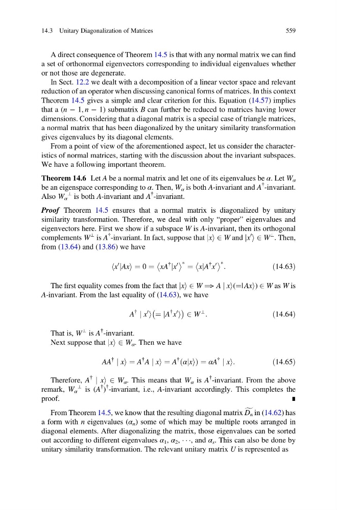
Theorem 14.6 Let A be a normal matrix and let one of its eigenvalues be α. Let W α
be an eigenspace corresponding to α. Then, W α is both A-invariant and A
{ -invariant.
Also W α
⊥ is both A-invariant and A
{ -invariant.
Proof Theorem 14.5 ensures that a normal matrix is diagonalized by unitary
similarity transformation. Therefore, we deal with only “proper” eigenvalues and
eigenvectors here. First we show if a subspace W is A-invariant, then its orthogonal
complements W
⊥ is A
{ -invariant. In fact, suppose that jxi 2 W and jx
0
i 2 W
⊥ . Then,
from (13.64) and (13.86) we have
x
0
jAx
h
i¼ 0 ¼ xA
{
jx
0
à ¼ xjA
{ x
0
à :
ð14:63Þ
The first equality comes from the fact that jxi 2 W ⟹ A j xi(¼| Axi) 2 W as W is
A-invariant. From the last equality of (14.63), we have
A
{
j x
0
i ¼ jA
{ x
0
i
À
Á 2 W
⊥
:
ð14:64Þ
That is, W
⊥ is A
{ -invariant.
Next suppose that jxi 2 W α . Then we have
AA
{
j xi ¼ A
{ A j xi ¼ A
{
αjxi
ð
Þ ¼ αA
{
j xi:
ð14:65Þ
Therefore, A
{
j xi 2 W α . This means that W α is A
{ -invariant. From the above
remark, W α
⊥ is (A
{ )
{ -invariant, i.e., A-invariant accordingly. This completes the
proof.
∎
From Theorem 14.5, we know that the resulting diagonal matrix f
D n in (14.62) has
a form with n eigenvalues (α n ) some of which may be multiple roots arranged in
diagonal elements. After diagonalizing the matrix, those eigenvalues can be sorted
out according to different eigenvalues α 1 , α 2 , Á Á Á, and α s . This can also be done by
unitary similarity transformation. The relevant unitary matrix U is represented as
14.3 Unitary Diagonalization of Matrices
559
a set of orthonormal eigenvectors corresponding to individual eigenvalues whether
or not those are degenerate.
In Sect. 12.2 we dealt with a decomposition of a linear vector space and relevant
reduction of an operator when discussing canonical forms of matrices. In this context
Theorem 14.5 gives a simple and clear criterion for this. Equation (14.57) implies
that a (n À 1, n À 1) submatrix B can further be reduced to matrices having lower
dimensions. Considering that a diagonal matrix is a special case of triangle matrices,
a normal matrix that has been diagonalized by the unitary similarity transformation
gives eigenvalues by its diagonal elements.
From a point of view of the aforementioned aspect, let us consider the characteristics of normal matrices, starting with the discussion about the invariant subspaces.
We have a following important theorem.
Theorem 14.6 Let A be a normal matrix and let one of its eigenvalues be α. Let W α
be an eigenspace corresponding to α. Then, W α is both A-invariant and A
{ -invariant.
Also W α
⊥ is both A-invariant and A
{ -invariant.
Proof Theorem 14.5 ensures that a normal matrix is diagonalized by unitary
similarity transformation. Therefore, we deal with only “proper” eigenvalues and
eigenvectors here. First we show if a subspace W is A-invariant, then its orthogonal
complements W
⊥ is A
{ -invariant. In fact, suppose that jxi 2 W and jx
0
i 2 W
⊥ . Then,
from (13.64) and (13.86) we have
x
0
jAx
h
i¼ 0 ¼ xA
{
jx
0
à ¼ xjA
{ x
0
à :
ð14:63Þ
The first equality comes from the fact that jxi 2 W ⟹ A j xi(¼| Axi) 2 W as W is
A-invariant. From the last equality of (14.63), we have
A
{
j x
0
i ¼ jA
{ x
0
i
À
Á 2 W
⊥
:
ð14:64Þ
That is, W
⊥ is A
{ -invariant.
Next suppose that jxi 2 W α . Then we have
AA
{
j xi ¼ A
{ A j xi ¼ A
{
αjxi
ð
Þ ¼ αA
{
j xi:
ð14:65Þ
Therefore, A
{
j xi 2 W α . This means that W α is A
{ -invariant. From the above
remark, W α
⊥ is (A
{ )
{ -invariant, i.e., A-invariant accordingly. This completes the
proof.
∎
From Theorem 14.5, we know that the resulting diagonal matrix f
D n in (14.62) has
a form with n eigenvalues (α n ) some of which may be multiple roots arranged in
diagonal elements. After diagonalizing the matrix, those eigenvalues can be sorted
out according to different eigenvalues α 1 , α 2 , Á Á Á, and α s . This can also be done by
unitary similarity transformation. The relevant unitary matrix U is represented as
14.3 Unitary Diagonalization of Matrices
559