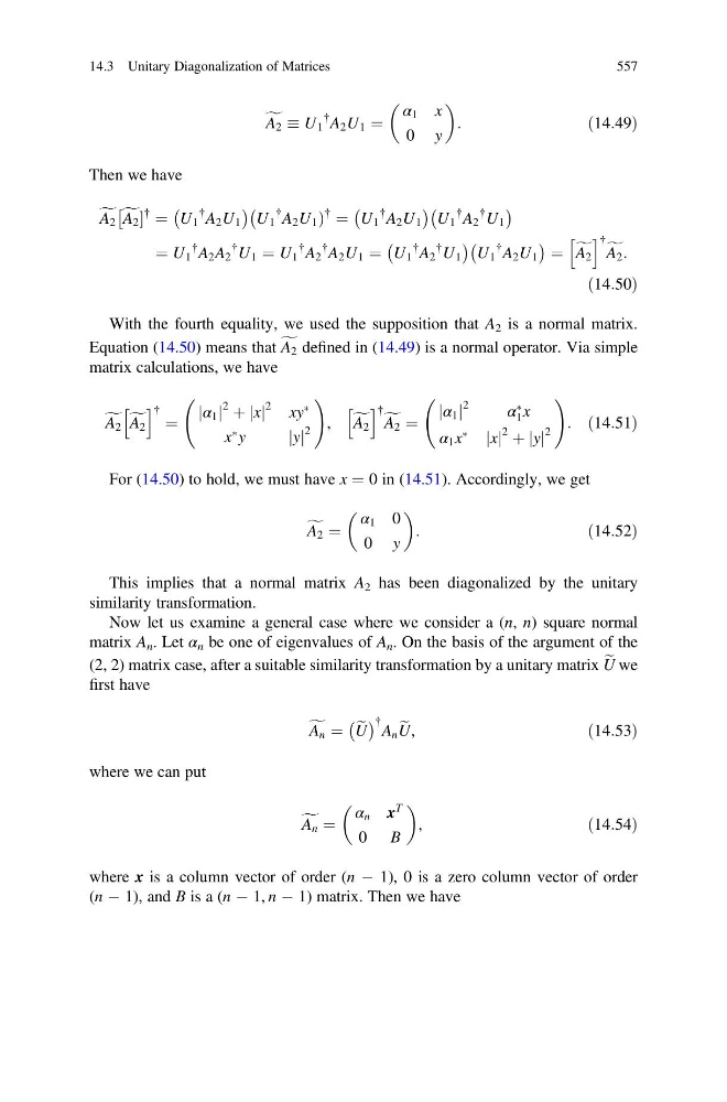
f A 2 U 1
{ A 2 U 1 ¼
α 1 x
0 y
:
ð14:49Þ
Then we have
f
A 2
 f
A 2 Š
{
¼ U 1
{ A 2 U 1
À
Á À
U 1
{ A 2 U 1 Þ
{
¼ U 1
{ A 2 U 1
À
Á
U 1
{ A 2
{ U 1
À
Á
¼ U 1
{ A 2 A 2
{ U 1 ¼ U 1
{ A 2
{ A 2 U 1 ¼ U 1
{ A 2
{ U 1
À
Á
U 1
{ A 2 U 1
À
Á ¼ f A 2
h i { f
A 2 :
ð14:50Þ
With the fourth equality, we used the supposition that A 2 is a normal matrix.
Equation (14.50) means that f A 2 defined in (14.49) is a normal operator. Via simple
matrix calculations, we have
f A 2 f A 2
h i { ¼
α 1
j j
2 þ x
j j
2
xy
Ã
x
à y
y
j j
2
!
, f A 2
h i { f A 2 ¼
α 1
j j
2
α
Ã
1 x
α 1 x
Ã
x
j j
2 þ y
j j
2
!
: ð14:51Þ
For (14.50) to hold, we must have x ¼ 0 in (14.51). Accordingly, we get
f A 2 ¼
α 1 0
0 y
:
ð14:52Þ
This implies that a normal matrix A 2 has been diagonalized by the unitary
similarity transformation.
Now let us examine a general case where we consider a (n, n) square normal
matrix A n . Let α n be one of eigenvalues of A n . On the basis of the argument of the
(2, 2) matrix case, after a suitable similarity transformation by a unitary matrix e
U we
first have
f
A n ¼ e
U
À Á { A n e
U,
ð14:53Þ
where we can put
f
A n ¼
α n x
T
0 B
,
ð14:54Þ
where x is a column vector of order (n À 1), 0 is a zero column vector of order
(n À 1), and B is a (n À 1, n À 1) matrix. Then we have
14.3 Unitary Diagonalization of Matrices
557