

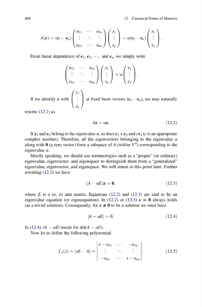
A x
ð Þ ¼ e 1 Á Á Áe n
ð
Þ
a 11 Á Á Á a 1n
⋮ ⋱ ⋮
a n1 Á Á Á a nn
0
B
@
1
C
A
x 1
⋮
x n
0
B
@
1
C
A ¼ α e 1 Á Á Áe n
ð
Þ
x 1
⋮
x n
0
B
@
1
C
A:
From linear dependence of e 1 , e 2 , Á Á Á, and e n , we simply write
a 11 Á Á Á a 1n
⋮ ⋱ ⋮
a n1 Á Á Á a nn
0
B
@
1
C
A
x 1
⋮
x n
0
B
@
1
C
A ¼ α
x 1
⋮
x n
0
B
@
1
C
A:
If we identify x with
x 1
⋮
x n
0
B
@
1
C
A at fixed basis vectors (e 1 Á Á Áe n ), we may naturally
rewrite (12.1) as
Ax ¼ αx:
ð12:2Þ
If x 1 and x 2 belong to the eigenvalue α, so does x 1 + x 2 and cx 1 (c is an appropriate
complex number). Therefore, all the eigenvectors belonging to the eigenvalue α
along with 0 (a zero vector) form a subspace of A (within V
n ) corresponding to the
eigenvalue α.
Strictly speaking, we should use terminologies such as a “proper” (or ordinary)
eigenvalue, eigenvector, and eigenspace to distinguish them from a “generalized”
eigenvalue, eigenvector, and eigenspace. We will return to this point later. Further
rewriting (12.2) we have
A À αE
ð
Þx ¼ 0,
ð12:3Þ
where E is a (n, n) unit matrix. Equations (12.2) and (12.3) are said to be an
eigenvalue equation (or eigenequation). In (12.2) or (12.3) x = 0 always holds
(as a trivial solution). Consequently, for x ≠ 0 to be a solution we must have
A À αE
j
j¼ 0,
ð12:4Þ
In (12.4), |A À αE| stands for det(A À αE).
Now let us define the following polynomial:
f A x
ð Þ ¼ xE À A
j
j¼
x À a 11 Á Á Á Àa 1n
⋮
⋱
⋮
Àa n1 Á Á Á x À a nn
:
ð12:5Þ
460
12 Canonical Forms of Matrices
ð Þ ¼ e 1 Á Á Áe n
ð
Þ
a 11 Á Á Á a 1n
⋮ ⋱ ⋮
a n1 Á Á Á a nn
0
B
@
1
C
A
x 1
⋮
x n
0
B
@
1
C
A ¼ α e 1 Á Á Áe n
ð
Þ
x 1
⋮
x n
0
B
@
1
C
A:
From linear dependence of e 1 , e 2 , Á Á Á, and e n , we simply write
a 11 Á Á Á a 1n
⋮ ⋱ ⋮
a n1 Á Á Á a nn
0
B
@
1
C
A
x 1
⋮
x n
0
B
@
1
C
A ¼ α
x 1
⋮
x n
0
B
@
1
C
A:
If we identify x with
x 1
⋮
x n
0
B
@
1
C
A at fixed basis vectors (e 1 Á Á Áe n ), we may naturally
rewrite (12.1) as
Ax ¼ αx:
ð12:2Þ
If x 1 and x 2 belong to the eigenvalue α, so does x 1 + x 2 and cx 1 (c is an appropriate
complex number). Therefore, all the eigenvectors belonging to the eigenvalue α
along with 0 (a zero vector) form a subspace of A (within V
n ) corresponding to the
eigenvalue α.
Strictly speaking, we should use terminologies such as a “proper” (or ordinary)
eigenvalue, eigenvector, and eigenspace to distinguish them from a “generalized”
eigenvalue, eigenvector, and eigenspace. We will return to this point later. Further
rewriting (12.2) we have
A À αE
ð
Þx ¼ 0,
ð12:3Þ
where E is a (n, n) unit matrix. Equations (12.2) and (12.3) are said to be an
eigenvalue equation (or eigenequation). In (12.2) or (12.3) x = 0 always holds
(as a trivial solution). Consequently, for x ≠ 0 to be a solution we must have
A À αE
j
j¼ 0,
ð12:4Þ
In (12.4), |A À αE| stands for det(A À αE).
Now let us define the following polynomial:
f A x
ð Þ ¼ xE À A
j
j¼
x À a 11 Á Á Á Àa 1n
⋮
⋱
⋮
Àa n1 Á Á Á x À a nn
:
ð12:5Þ
460
12 Canonical Forms of Matrices