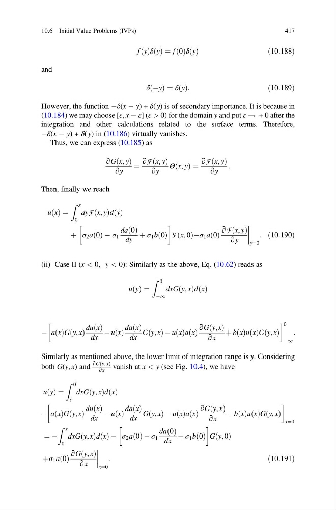
f y
ð Þδ y
ð Þ ¼ f 0
ð Þδ y
ð Þ
ð10:188Þ
and
δ Ày
ð Þ ¼ δ y
ð Þ:
ð10:189Þ
However, the function Àδ(x À y) + δ( y) is of secondary importance. It is because in
(10.184) we may choose [ε, x À ε] (ε > 0) for the domain y and put ε ! + 0 after the
integration and other calculations related to the surface terms. Therefore,
Àδ(x À y) + δ( y) in (10.186) virtually vanishes.
Thus, we can express (10.185) as
∂G x, y
ð Þ
∂y
¼
∂F x, y
ð Þ
∂y
Θ x, y
ð Þ ¼
∂F x, y
ð Þ
∂y
:
Then, finally we reach
u x
ð Þ ¼
Z x
0
dyF x, y
ð Þd y
ð Þ
þ σ 2 a 0
ð Þ À σ 1
da 0
ð Þ
dy
þ σ 1 b 0
ð Þ
!
F x, 0
ð ÞÀσ 1 a 0
ð Þ
∂F x, y
ð Þ
∂y
y¼0
: ð10:190Þ
(ii) Case II (x < 0, y < 0): Similarly as the above, Eq. (10.62) reads as
u y
ð Þ ¼
Z 0
À1
dxG y, x
ð Þd x
ð Þ
À a x
ð ÞG y, x
ð Þ
du x
ð Þ
dx
À u x
ð Þ
da x
ð Þ
dx
G y, x
ð ÞÀu x
ð Þa x
ð Þ
∂G y, x
ð Þ
∂x
þ b x
ð Þu x
ð ÞG y, x
ð Þ
! 0
À1
:
Similarly as mentioned above, the lower limit of integration range is y. Considering
both G(y, x) and
∂G y, x
ð Þ
∂x
vanish at x < y (see Fig. 10.4), we have
u y
ð Þ ¼
Z 0
y
dxG y, x
ð Þd x
ð Þ
À a x
ð ÞG y, x
ð Þ
du x
ð Þ
dx
À u x
ð Þ
da x
ð Þ
dx
G y, x
ð ÞÀu x
ð Þa x
ð Þ
∂G y, x
ð Þ
∂x
þ b x
ð Þu x
ð ÞG y, x
ð Þ
!
x¼0
¼ À
Z y
0
dxG y, x
ð Þd x
ð Þ À σ 2 a 0
ð Þ À σ 1
da 0
ð Þ
dx
þ σ 1 b 0
ð Þ
!
G y, 0
ð Þ
þσ 1 a 0
ð Þ
∂G y, x
ð Þ
∂x
x¼0
:
ð10:191Þ
10.6 Initial Value Problems (IVPs)
417