Note that in the above we used L x
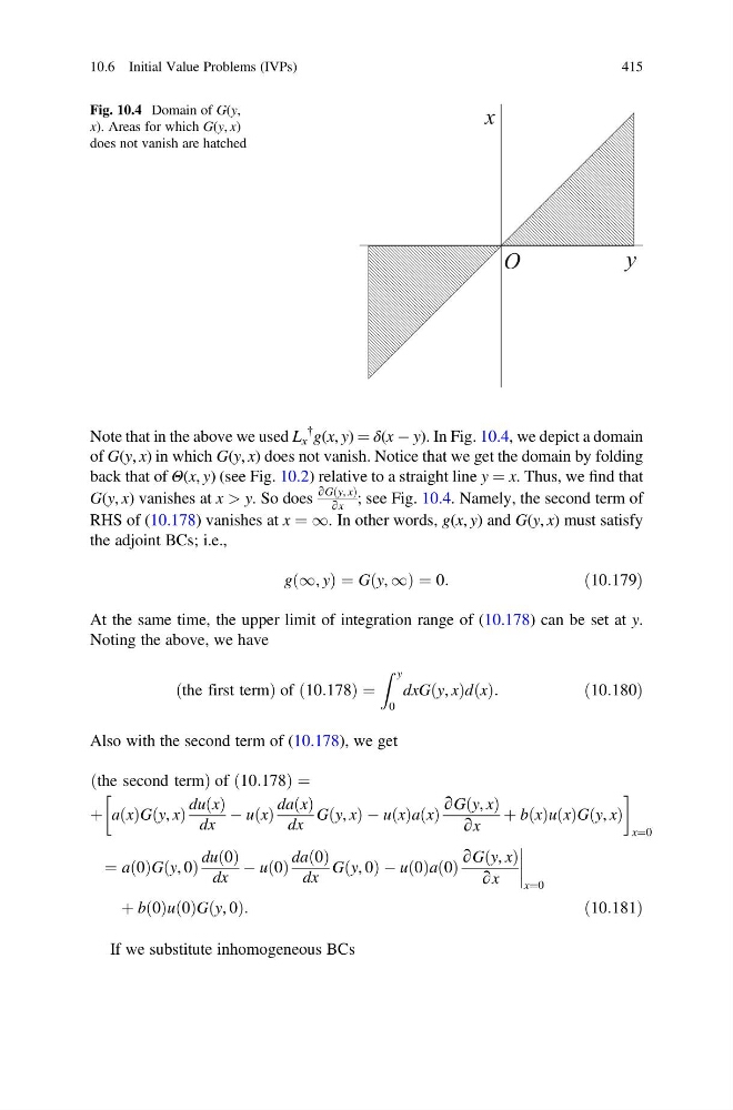
{ g(x, y) ¼ δ(x À y). In Fig. 10.4, we depict a domain
of G(y, x) in which G(y, x) does not vanish. Notice that we get the domain by folding
back that of Θ(x, y) (see Fig. 10.2) relative to a straight line y ¼ x. Thus, we find that
G(y, x) vanishes at x > y. So does
∂G y, x
ð Þ
∂x
; see Fig. 10.4. Namely, the second term of
RHS of (10.178) vanishes at x ¼ 1. In other words, g(x, y) and G(y, x) must satisfy
the adjoint BCs; i.e.,
g 1, y
ð
Þ¼G y, 1
ð
Þ¼0:
ð10:179Þ
At the same time, the upper limit of integration range of (10.178) can be set at y.
Noting the above, we have
the first term
ð
Þof 10:178
ð
Þ¼
Z y
0
dxG y, x
ð Þd x
ð Þ:
ð10:180Þ
Also with the second term of (10.178), we get
the second term
ð
Þ of 10:178
ð
Þ¼
þ a x
ð ÞG y, x
ð Þ
du x
ð Þ
dx
À u x
ð Þ
da x
ð Þ
dx
G y, x
ð ÞÀu x
ð Þa x
ð Þ
∂G y, x
ð Þ
∂x
þ b x
ð Þu x
ð ÞG y, x
ð Þ
!
x¼0
¼ a 0
ð ÞG y, 0
ð Þ
du 0
ð Þ
dx
À u 0
ð Þ
da 0
ð Þ
dx
G y, 0
ð ÞÀu 0
ð Þa 0
ð Þ
∂G y, x
ð Þ
∂x
x¼0
þ b 0
ð Þu 0
ð ÞG y, 0
ð Þ:
ð10:181Þ
If we substitute inhomogeneous BCs
x
y
O
Fig. 10.4 Domain of G(y,
x). Areas for which G(y, x)
does not vanish are hatched
10.6 Initial Value Problems (IVPs)
415