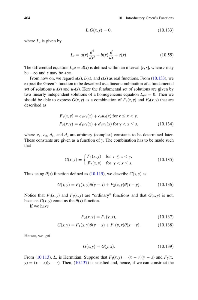
L x G x, y
ð Þ ¼ 0,
ð10:133Þ
where L x is given by
L x ¼ a x
ð Þ
d
2
dx 2 þ b x
ð Þ
d
dx
þ c x
ð Þ:
ð10:55Þ
The differential equation L x u ¼ d(x) is defined within an interval [r, s], where r may
be À1 and s may be +1.
From now on, we regard a(x), b(x), and c(x) as real functions. From (10.133), we
expect the Green’s function to be described as a linear combination of a fundamental
set of solutions u 1 (x) and u 2 (x). Here the fundamental set of solutions are given by
two linearly independent solutions of a homogeneous equation L x u ¼ 0. Then we
should be able to express G(x, y) as a combination of F 1 (x, y) and F 2 (x, y) that are
described as
F 1 x, y
ð Þ ¼ c 1 u 1 x
ð Þ þ c 2 u 2 x
ð Þ for r x < y,
F 2 x, y
ð Þ ¼ d 1 u 1 x
ð Þ þ d 2 u 2 x
ð Þ for y < x s,
ð10:134Þ
where c 1 , c 2 , d 1 , and d 2 are arbitrary (complex) constants to be determined later.
These constants are given as a function of y. The combination has to be made such
that
G x, y
ð Þ ¼
F 1 x, y
ð Þ for r x < y,
F 2 x, y
ð Þ for y < x s:
&
ð10:135Þ
Thus using θ(x) function defined as (10.119), we describe G(x, y) as
G x, y
ð Þ ¼ F 1 x, y
ð Þθ y À x
ð
ÞþF 2 x, y
ð Þθ x À y
ð
Þ:
ð10:136Þ
Notice that F 1 (x, y) and F 2 (x, y) are “ordinary” functions and that G(x, y) is not,
because G(x, y) contains the θ(x) function.
If we have
F 2 x, y
ð Þ ¼ F 1 y, x
ð Þ,
ð10:137Þ
G x, y
ð Þ ¼ F 1 x, y
ð Þθ y À x
ð
ÞþF 1 y, x
ð Þθ x À y
ð
Þ:
ð10:138Þ
Hence, we get
G x, y
ð Þ ¼ G y, x
ð Þ:
ð10:139Þ
From (10.113), L x is Hermitian. Suppose that F 1 (x, y) ¼ (x À r)(y À s) and F 2 (x,
y) ¼ (x À s)(y À r). Then, (10.137) is satisfied and, hence, if we can construct the
404
10 Introductory Green’s Functions