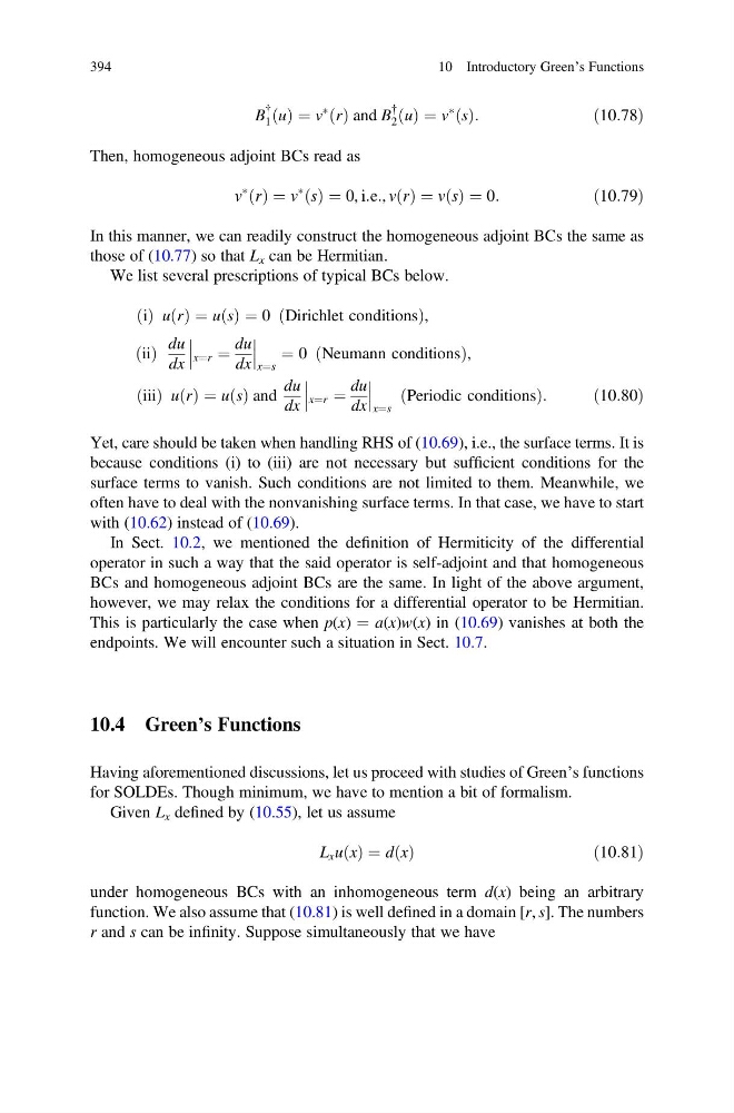
B
{
1 u
ð Þ ¼ v
à r
ð Þ and B
{
2 u
ð Þ ¼ v
à s
ð Þ:
ð10:78Þ
Then, homogeneous adjoint BCs read as
v
à r
ð Þ ¼ v
à s
ð Þ ¼ 0, i:e:, v r
ð Þ ¼ v s
ð Þ ¼ 0:
ð10:79Þ
In this manner, we can readily construct the homogeneous adjoint BCs the same as
those of (10.77) so that L x can be Hermitian.
We list several prescriptions of typical BCs below.
i
ð Þ u r
ð Þ ¼ u s
ð Þ ¼ 0 Dirichlet conditions
ð
Þ ,
ii
ð Þ
du
dx
x¼r ¼
du
dx
x¼s
¼ 0 Neumann conditions
ð
Þ ,
iii
ð Þ u r
ð Þ ¼ u s
ð Þ and
du
dx
x¼r ¼
du
dx
x¼s
Periodic conditions
ð
Þ :
ð10:80Þ
Yet, care should be taken when handling RHS of (10.69), i.e., the surface terms. It is
because conditions (i) to (iii) are not necessary but sufficient conditions for the
surface terms to vanish. Such conditions are not limited to them. Meanwhile, we
often have to deal with the nonvanishing surface terms. In that case, we have to start
with (10.62) instead of (10.69).
In Sect. 10.2, we mentioned the definition of Hermiticity of the differential
operator in such a way that the said operator is self-adjoint and that homogeneous
BCs and homogeneous adjoint BCs are the same. In light of the above argument,
however, we may relax the conditions for a differential operator to be Hermitian.
This is particularly the case when p(x) ¼ a(x)w(x) in (10.69) vanishes at both the
endpoints. We will encounter such a situation in Sect. 10.7.
10.4 Green’s Functions
Having aforementioned discussions, let us proceed with studies of Green’s functions
for SOLDEs. Though minimum, we have to mention a bit of formalism.
Given L x defined by (10.55), let us assume
L x u x
ð Þ ¼ d x
ð Þ
ð10:81Þ
under homogeneous BCs with an inhomogeneous term d(x) being an arbitrary
function. We also assume that (10.81) is well defined in a domain [r, s]. The numbers
r and s can be infinity. Suppose simultaneously that we have
394
10 Introductory Green’s Functions