

If d(x) ¼ 0, the differential equation is said to be homogeneous; otherwise it is called
inhomogeneous. Equation (10.1) is a linear function of u and its derivatives.
Likewise, we have a SOLDE such that
a x
ð Þ
d
2 u
dx 2 þ b x
ð Þ
du
dx
þ c x
ð Þu ¼ d x
ð Þ:
ð10:2Þ
In (10.2) we assume that the variable x is real. The equation can be solved under
appropriate boundary conditions (BCs). A general form of BCs is described as
B 1 u
ð Þ ¼ α 1 u a
ð Þ þ β 1
du
dx
x¼a þ γ 1 u b
ð Þ þ δ 1
du
dx
x¼b
¼ σ 1 ,
ð10:3Þ
B 2 u
ð Þ ¼ α 2 u a
ð Þ þ β 2
du
dx
x¼a þ γ 2 u b
ð Þ þ δ 2
du
dx
x¼b
¼ σ 2 ,
ð10:4Þ
where α 1 , β 1 , γ 1 , δ 1 σ 1 , etc. are real constants; u(x) is defined in an interval [a, b],
where a and b can be infinity (i.e., Æ1). The LHS of B 1 (u) and B 2 (u) are referred to
as boundary functionals [1, 2]. If σ 1 ¼ σ 2 ¼ 0, the BCs are called homogeneous;
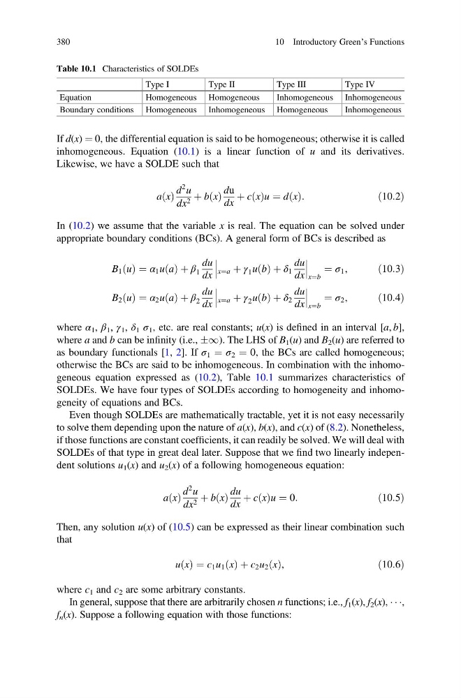
otherwise the BCs are said to be inhomogeneous. In combination with the inhomogeneous equation expressed as (10.2), Table 10.1 summarizes characteristics of
SOLDEs. We have four types of SOLDEs according to homogeneity and inhomogeneity of equations and BCs.
Even though SOLDEs are mathematically tractable, yet it is not easy necessarily
to solve them depending upon the nature of a(x), b(x), and c(x) of (8.2). Nonetheless,
if those functions are constant coefficients, it can readily be solved. We will deal with
SOLDEs of that type in great deal later. Suppose that we find two linearly independent solutions u 1 (x) and u 2 (x) of a following homogeneous equation:
a x
ð Þ
d
2 u
dx 2 þ b x
ð Þ
du
dx
þ c x
ð Þu ¼ 0:
ð10:5Þ
Then, any solution u(x) of (10.5) can be expressed as their linear combination such
that
u x
ð Þ ¼ c 1 u 1 x
ð Þ þ c 2 u 2 x
ð Þ,
ð10:6Þ
where c 1 and c 2 are some arbitrary constants.
In general, suppose that there are arbitrarily chosen n functions; i.e., f 1 (x), f 2 (x), Á Á Á,
f n (x). Suppose a following equation with those functions:
Table 10.1 Characteristics of SOLDEs
Type I
Type II
Type III
Type IV
Equation
Homogeneous Homogeneous
Inhomogeneous Inhomogeneous
Boundary conditions Homogeneous Inhomogeneous Homogeneous
Inhomogeneous
380
10 Introductory Green’s Functions
inhomogeneous. Equation (10.1) is a linear function of u and its derivatives.
Likewise, we have a SOLDE such that
a x
ð Þ
d
2 u
dx 2 þ b x
ð Þ
du
dx
þ c x
ð Þu ¼ d x
ð Þ:
ð10:2Þ
In (10.2) we assume that the variable x is real. The equation can be solved under
appropriate boundary conditions (BCs). A general form of BCs is described as
B 1 u
ð Þ ¼ α 1 u a
ð Þ þ β 1
du
dx
x¼a þ γ 1 u b
ð Þ þ δ 1
du
dx
x¼b
¼ σ 1 ,
ð10:3Þ
B 2 u
ð Þ ¼ α 2 u a
ð Þ þ β 2
du
dx
x¼a þ γ 2 u b
ð Þ þ δ 2
du
dx
x¼b
¼ σ 2 ,
ð10:4Þ
where α 1 , β 1 , γ 1 , δ 1 σ 1 , etc. are real constants; u(x) is defined in an interval [a, b],
where a and b can be infinity (i.e., Æ1). The LHS of B 1 (u) and B 2 (u) are referred to
as boundary functionals [1, 2]. If σ 1 ¼ σ 2 ¼ 0, the BCs are called homogeneous;
otherwise the BCs are said to be inhomogeneous. In combination with the inhomogeneous equation expressed as (10.2), Table 10.1 summarizes characteristics of
SOLDEs. We have four types of SOLDEs according to homogeneity and inhomogeneity of equations and BCs.
Even though SOLDEs are mathematically tractable, yet it is not easy necessarily
to solve them depending upon the nature of a(x), b(x), and c(x) of (8.2). Nonetheless,
if those functions are constant coefficients, it can readily be solved. We will deal with
SOLDEs of that type in great deal later. Suppose that we find two linearly independent solutions u 1 (x) and u 2 (x) of a following homogeneous equation:
a x
ð Þ
d
2 u
dx 2 þ b x
ð Þ
du
dx
þ c x
ð Þu ¼ 0:
ð10:5Þ
Then, any solution u(x) of (10.5) can be expressed as their linear combination such
that
u x
ð Þ ¼ c 1 u 1 x
ð Þ þ c 2 u 2 x
ð Þ,
ð10:6Þ
where c 1 and c 2 are some arbitrary constants.
In general, suppose that there are arbitrarily chosen n functions; i.e., f 1 (x), f 2 (x), Á Á Á,
f n (x). Suppose a following equation with those functions:
Table 10.1 Characteristics of SOLDEs
Type I
Type II
Type III
Type IV
Equation
Homogeneous Homogeneous
Inhomogeneous Inhomogeneous
Boundary conditions Homogeneous Inhomogeneous Homogeneous
Inhomogeneous
380
10 Introductory Green’s Functions