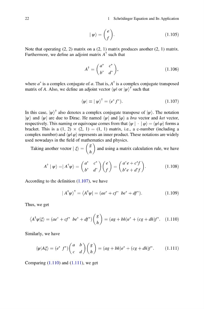
j ψi ¼
e
f
:
ð1:105Þ
Note that operating (2, 2) matrix on a (2, 1) matrix produces another (2, 1) matrix.
Furthermore, we define an adjoint matrix A
{ such that
A
{
¼
a
Ã
c
Ã
b
Ã
d
Ã
,
ð1:106Þ
where a
à is a complex conjugate of a. That is, A
{ is a complex conjugate transposed
matrix of A. Also, we define an adjoint vector hψ| or jψi
{ such that
ψj
h
j ψi
{ ¼ e
à f
Ã
ð
Þ:
ð1:107Þ
In this case, jψi
{ also denotes a complex conjugate transpose of jψi. The notation
jψi and hψj are due to Dirac. He named hψj and jφi a bra vector and ket vector,
respectively. This naming or equivoque comes from that hψ j Á j φi ¼ hψ| φi forms a
bracket. This is a (1, 2) Â (2, 1) ¼ (1, 1) matrix, i.e., a c-number (including a
complex number) and hψ| φi represents an inner product. These notations are widely
used nowadays in the field of mathematics and physics.
Taking another vector j ξi ¼
g
h
and using a matrix calculation rule, we have
A
{
j ψi ¼j A
{
ψi ¼
a
Ã
c
Ã
b
à d
Ã
e
f
¼
a
à e þ c
à f
b
à e þ d
à f
:
ð1:108Þ
According to the definition (1.107), we have
j A
{
ψi
{ ¼ A
{
ψj
¼ ae
Ã
þ cf
à be
Ã
þ df
Ã
ð
Þ :
ð1:109Þ
Thus, we get
A
{
ψjξi
¼ ae
Ã
þ cf
à be
Ã
þ df
Ã
ð
Þ
g
h
¼ ag þ bh
ð
Þ e
Ã
þ cg þ dh
ð
Þ f
Ã
: ð1:110Þ
Similarly, we have
ψjAξi
h
¼ e
à f
Ã
ð
Þ
a b
c d
g
h
¼ ag þ bh
ð
Þ e
Ã
þ cg þ dh
ð
Þ f
Ã
:
ð1:111Þ
Comparing (1.110) and (1.111), we get
22
1 Schrödinger Equation and Its Application