

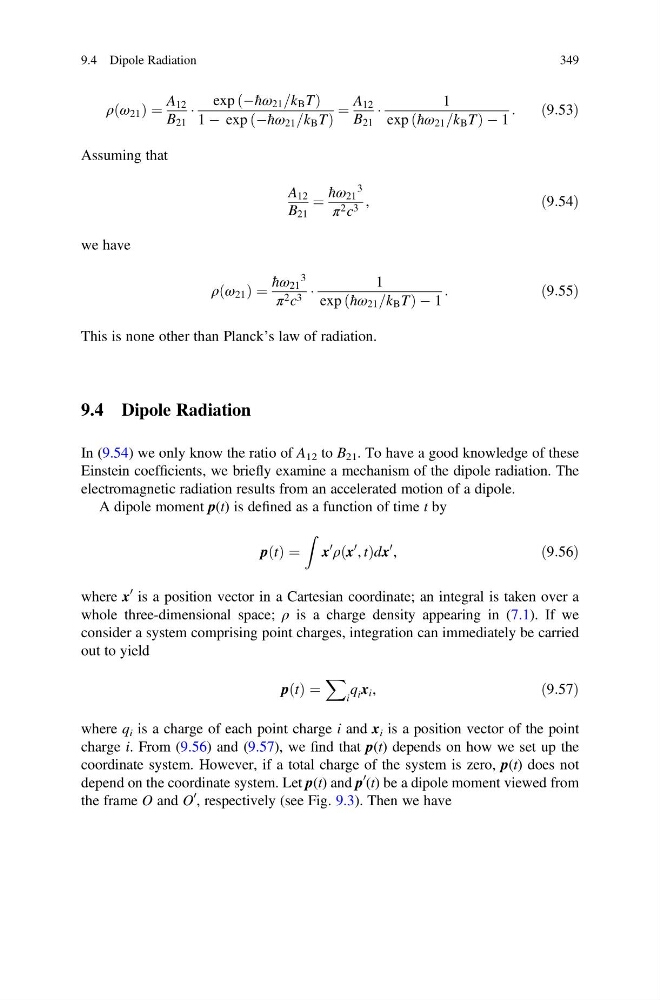
ρ ω 21
ð Þ ¼
A 12
B 21
Á
exp Àħω 21 =k B T
ð
Þ
1 À exp Àħω 21 =k B T
ð
Þ
¼
A 12
B 21
Á
1
exp ħω 21 =k B T
ð
ÞÀ1
:
ð9:53Þ
Assuming that
A 12
B 21
¼
ħω 21
3
π 2 c 3 ,
ð9:54Þ
we have
ρ ω 21
ð Þ ¼
ħω 21
3
π 2 c 3 Á
1
exp ħω 21 =k B T
ð
ÞÀ1
:
ð9:55Þ
This is none other than Planck’s law of radiation.
9.4 Dipole Radiation
In (9.54) we only know the ratio of A 12 to B 21 . To have a good knowledge of these
Einstein coefficients, we briefly examine a mechanism of the dipole radiation. The
electromagnetic radiation results from an accelerated motion of a dipole.
A dipole moment p(t) is defined as a function of time t by
p t
ð Þ ¼
Z
x
0
ρ x
0 , t
ð Þdx
0 ,
ð9:56Þ
where x
0 is a position vector in a Cartesian coordinate; an integral is taken over a
whole three-dimensional space; ρ is a charge density appearing in (7.1). If we
consider a system comprising point charges, integration can immediately be carried
out to yield
p t
ð Þ ¼
X
i
q i x i ,
ð9:57Þ
where q i is a charge of each point charge i and x i is a position vector of the point
charge i. From (9.56) and (9.57), we find that p(t) depends on how we set up the
coordinate system. However, if a total charge of the system is zero, p(t) does not
depend on the coordinate system. Let p(t) and p
0
(t) be a dipole moment viewed from
the frame O and O
0 , respectively (see Fig. 9.3). Then we have
9.4 Dipole Radiation
349
ð Þ ¼
A 12
B 21
Á
exp Àħω 21 =k B T
ð
Þ
1 À exp Àħω 21 =k B T
ð
Þ
¼
A 12
B 21
Á
1
exp ħω 21 =k B T
ð
ÞÀ1
:
ð9:53Þ
Assuming that
A 12
B 21
¼
ħω 21
3
π 2 c 3 ,
ð9:54Þ
we have
ρ ω 21
ð Þ ¼
ħω 21
3
π 2 c 3 Á
1
exp ħω 21 =k B T
ð
ÞÀ1
:
ð9:55Þ
This is none other than Planck’s law of radiation.
9.4 Dipole Radiation
In (9.54) we only know the ratio of A 12 to B 21 . To have a good knowledge of these
Einstein coefficients, we briefly examine a mechanism of the dipole radiation. The
electromagnetic radiation results from an accelerated motion of a dipole.
A dipole moment p(t) is defined as a function of time t by
p t
ð Þ ¼
Z
x
0
ρ x
0 , t
ð Þdx
0 ,
ð9:56Þ
where x
0 is a position vector in a Cartesian coordinate; an integral is taken over a
whole three-dimensional space; ρ is a charge density appearing in (7.1). If we
consider a system comprising point charges, integration can immediately be carried
out to yield
p t
ð Þ ¼
X
i
q i x i ,
ð9:57Þ
where q i is a charge of each point charge i and x i is a position vector of the point
charge i. From (9.56) and (9.57), we find that p(t) depends on how we set up the
coordinate system. However, if a total charge of the system is zero, p(t) does not
depend on the coordinate system. Let p(t) and p
0
(t) be a dipole moment viewed from
the frame O and O
0 , respectively (see Fig. 9.3). Then we have
9.4 Dipole Radiation
349