

1
X
d
2 X
dx 2 þ
1
Y
d
2 Y
dx 2 þ
1
Z
d
2 Z
dx 2 ¼
1
v 2
1
T
d
2 T
dt
2
¼ Àk
2
:
ð9:23Þ
Putting
1
X
d
2 X
dx 2 ¼ Àk
2
x ,
1
Y
d
2 Y
dx 2 ¼ Àk
2
y ,
1
Z
d
2 Z
dx 2 ¼ Àk
2
z ,
ð9:24Þ
we have
k
2
x þ k
2
y þ k
2
z ¼ k
2
:
ð9:25Þ
Then, we get a stationary wave solution as in the one-dimensional case such that
ψ x, t
ð Þ ¼ c sin k x x sin k y y sin k z z sin ωt:
ð9:26Þ
The BCs to be satisfied with X(x), Y( y), and Z(z) are
k x L ¼ m x π, k y L ¼ m y π, k z L ¼ m z π m x , m y , m z ¼ 1, 2, Á Á Á
À
Á :
ð9:27Þ
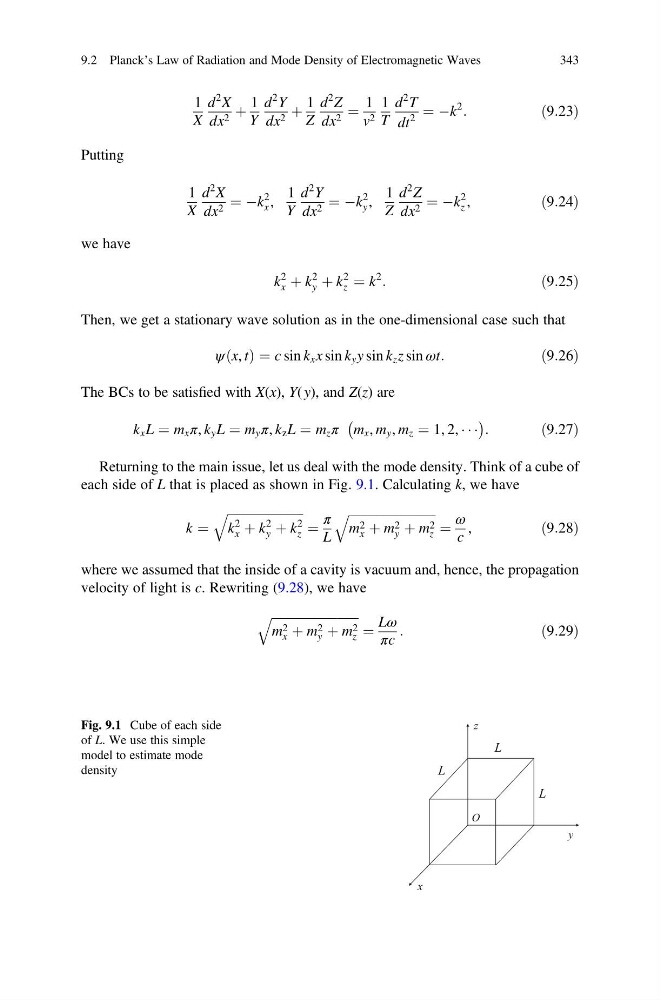
Returning to the main issue, let us deal with the mode density. Think of a cube of
each side of L that is placed as shown in Fig. 9.1. Calculating k, we have
k ¼
ffiffiffiffiffiffiffiffiffiffiffiffiffiffiffiffiffiffiffiffiffiffiffiffi ffi
k
2
x þ k
2
y þ k
2
z
q
¼
π
L
ffiffiffiffiffiffiffiffiffiffiffiffiffiffiffiffiffiffiffiffiffiffiffiffiffiffiffiffi
m 2
x þ m 2
y þ m 2
z
q
¼
ω
c
,
ð9:28Þ
where we assumed that the inside of a cavity is vacuum and, hence, the propagation
velocity of light is c. Rewriting (9.28), we have
ffiffiffiffiffiffiffiffiffiffiffiffiffiffiffiffiffiffiffiffiffiffiffiffiffiffiffiffi
m 2
x þ m 2
y þ m 2
z
q
¼
Lω
πc
:
ð9:29Þ
y
x
z
L
L
L
O
Fig. 9.1 Cube of each side
of L. We use this simple
model to estimate mode
density
9.2 Planck’s Law of Radiation and Mode Density of Electromagnetic Waves
343
X
d
2 X
dx 2 þ
1
Y
d
2 Y
dx 2 þ
1
Z
d
2 Z
dx 2 ¼
1
v 2
1
T
d
2 T
dt
2
¼ Àk
2
:
ð9:23Þ
Putting
1
X
d
2 X
dx 2 ¼ Àk
2
x ,
1
Y
d
2 Y
dx 2 ¼ Àk
2
y ,
1
Z
d
2 Z
dx 2 ¼ Àk
2
z ,
ð9:24Þ
we have
k
2
x þ k
2
y þ k
2
z ¼ k
2
:
ð9:25Þ
Then, we get a stationary wave solution as in the one-dimensional case such that
ψ x, t
ð Þ ¼ c sin k x x sin k y y sin k z z sin ωt:
ð9:26Þ
The BCs to be satisfied with X(x), Y( y), and Z(z) are
k x L ¼ m x π, k y L ¼ m y π, k z L ¼ m z π m x , m y , m z ¼ 1, 2, Á Á Á
À
Á :
ð9:27Þ
Returning to the main issue, let us deal with the mode density. Think of a cube of
each side of L that is placed as shown in Fig. 9.1. Calculating k, we have
k ¼
ffiffiffiffiffiffiffiffiffiffiffiffiffiffiffiffiffiffiffiffiffiffiffiffi ffi
k
2
x þ k
2
y þ k
2
z
q
¼
π
L
ffiffiffiffiffiffiffiffiffiffiffiffiffiffiffiffiffiffiffiffiffiffiffiffiffiffiffiffi
m 2
x þ m 2
y þ m 2
z
q
¼
ω
c
,
ð9:28Þ
where we assumed that the inside of a cavity is vacuum and, hence, the propagation
velocity of light is c. Rewriting (9.28), we have
ffiffiffiffiffiffiffiffiffiffiffiffiffiffiffiffiffiffiffiffiffiffiffiffiffiffiffiffi
m 2
x þ m 2
y þ m 2
z
q
¼
Lω
πc
:
ð9:29Þ
y
x
z
L
L
L
O
Fig. 9.1 Cube of each side
of L. We use this simple
model to estimate mode
density
9.2 Planck’s Law of Radiation and Mode Density of Electromagnetic Waves
343