

b 1 ¼ kx À ωt and b 2 ¼ Àkx À ωt,
ð8:187Þ
where the former equation represents a forward wave, whereas the latter a backward
wave. Then we have
b 1 À b 2 ¼ 2kx:
ð8:188Þ
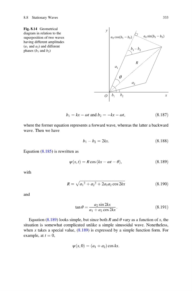
Equation (8.185) is rewritten as
ψ x, t
ð Þ ¼ R cos kx À ωt À θ
ð
Þ ,
ð8:189Þ
with
R ¼
ffiffiffiffiffiffiffiffiffiffiffiffiffiffiffiffiffiffiffiffiffiffiffiffiffiffiffiffiffiffiffiffiffiffiffiffiffiffiffiffiffiffiffiffiffiffiffiffiffiffi
a 1
2 þ a 2
2 þ 2a 1 a 2 cos 2kx
p
ð8:190Þ
and
tan θ ¼
a 2 sin 2kx
a 1 þ a 2 cos 2kx
:
ð8:191Þ
Equation (8.189) looks simple, but since both R and θ vary as a function of x, the
situation is somewhat complicated unlike a simple sinusoidal wave. Nonetheless,
when x takes a special value, (8.189) is expressed by a simple function form. For
example, at t ¼ 0,
ψ x, 0
ð Þ ¼ a 1 þ a 2
ð
Þcos kx:
x
y
θ
a 1
b 2
a 2
b 1
b 1 ‒ b 2
sin( − )
cos( − )
O
Fig. 8.14 Geometrical
diagram in relation to the
superposition of two waves
having different amplitudes
(a 1 and a 2 ) and different
phases (b 1 and b 2 )
8.8 Stationary Waves
333
ð8:187Þ
where the former equation represents a forward wave, whereas the latter a backward
wave. Then we have
b 1 À b 2 ¼ 2kx:
ð8:188Þ
Equation (8.185) is rewritten as
ψ x, t
ð Þ ¼ R cos kx À ωt À θ
ð
Þ ,
ð8:189Þ
with
R ¼
ffiffiffiffiffiffiffiffiffiffiffiffiffiffiffiffiffiffiffiffiffiffiffiffiffiffiffiffiffiffiffiffiffiffiffiffiffiffiffiffiffiffiffiffiffiffiffiffiffiffi
a 1
2 þ a 2
2 þ 2a 1 a 2 cos 2kx
p
ð8:190Þ
and
tan θ ¼
a 2 sin 2kx
a 1 þ a 2 cos 2kx
:
ð8:191Þ
Equation (8.189) looks simple, but since both R and θ vary as a function of x, the
situation is somewhat complicated unlike a simple sinusoidal wave. Nonetheless,
when x takes a special value, (8.189) is expressed by a simple function form. For
example, at t ¼ 0,
ψ x, 0
ð Þ ¼ a 1 þ a 2
ð
Þcos kx:
x
y
θ
a 1
b 2
a 2
b 1
b 1 ‒ b 2
sin( − )
cos( − )
O
Fig. 8.14 Geometrical
diagram in relation to the
superposition of two waves
having different amplitudes
(a 1 and a 2 ) and different
phases (b 1 and b 2 )
8.8 Stationary Waves
333