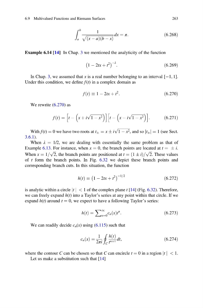
Z b
a
1
ffiffiffiffiffiffiffiffiffiffiffiffiffiffiffiffiffiffiffiffiffiffiffiffiffiffiffiffi ffi
x À a
ð
Þ b À x
ð
Þ
p
dx ¼ π:
ð6:268Þ
Example 6.14 [14] In Chap. 3 we mentioned the analyticity of the function
1 À 2tx þ t
2
À
Á Àλ :
ð6:269Þ
In Chap. 3, we assumed that x is a real number belonging to an interval [À1, 1].
Under this condition, we define f (t) in a complex domain as
f t
ð Þ 1 À 2tx þ t
2
:
ð6:270Þ
We rewrite (6.270) as
f t
ð Þ ¼ t À x þ i
ffiffiffiffiffiffiffiffiffiffiffiffi ffi
1 À x 2
p
h
i
t À x À i
ffiffiffiffiffiffiffiffiffiffiffiffi ffi
1 À x 2
p
h
i
:
ð6:271Þ
With f (t) ¼ 0 we have two roots at t Æ ¼ x Æ i
ffiffiffiffiffiffiffiffiffiffiffiffi ffi
1 À x 2
p
, and so jt Æ j ¼ 1 (see Sect.
3.6.1).
When λ ¼ 1/2, we are dealing with essentially the same problem as that of
Example 6.13. For instance, when x ¼ 0, the branch points are located at t ¼ Æ i.
When x ¼ 1=
ffiffi ffi
2
p
, the branch points are positioned at t ¼ 1 Æ i
ð
Þ=
ffiffi ffi
2
p
. These values
of t form the branch points. In Fig. 6.32 we depict these branch points and
corresponding branch cuts. In this situation, the function
h t
ð Þ 1 À 2tx þ t
2
À
Á À1=2
ð6:272Þ
is analytic within a circle jt j < 1 of the complex plane t [14] (Fig. 6.32). Therefore,
we can freely expand h(t) into a Taylor’s series at any point within that circle. If we
expand h(t) around t ¼ 0, we expect to have a following Taylor’s series:
h t
ð Þ ¼
X 1
n¼0
c n x
ð Þt
n
:
ð6:273Þ
We can readily decide c n (x) using (6.115) such that
c n x
ð Þ ¼
1
2πi
I
C
h t
ð Þ
t nþ1 dt,
ð6:274Þ
where the contour C can be chosen so that C can encircle t ¼ 0 in a region jt j < 1.
Let us make a substitution such that [14]
6.9 Multivalued Functions and Riemann Surfaces
263