

lim
R!1
I C ¼
Z 1
0
dx
1 þ x 3 þ
Z
Γ 1
dz
1 þ z 3 À e
2πi=3
Z 1
0
dr
1 þ r 3 :
ð6:186Þ
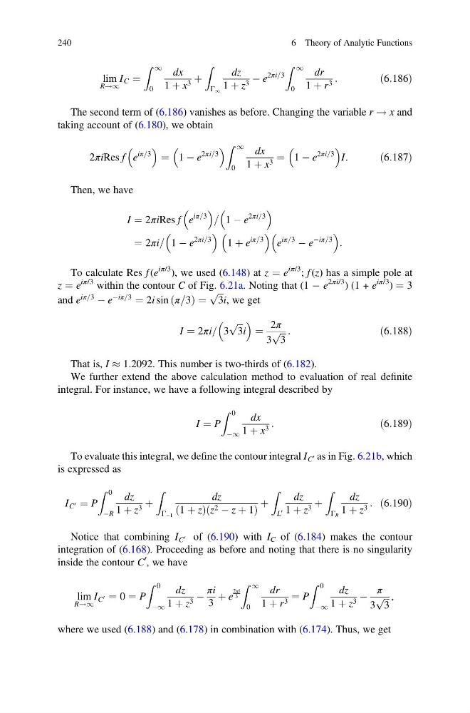
The second term of (6.186) vanishes as before. Changing the variable r ! x and
taking account of (6.180), we obtain
2πiRes f e
iπ=3
¼ 1 À e
2πi=3
Z 1
0
dx
1 þ x 3 ¼ 1 À e
2πi=3
I:
ð6:187Þ
Then, we have
I ¼ 2πiRes f e
iπ=3
= 1 À e
2πi=3
¼ 2πi= 1 À e
2πi=3
1 þ e
iπ=3
e
iπ=3
À e
Àiπ=3
:
To calculate Res f (e
iπ/3 ), we used (6.148) at z ¼ e
iπ/3 ; f (z) has a simple pole at
z ¼ e
iπ/3 within the contour C of Fig. 6.21a. Noting that (1 À e
2πi/3 ) (1 + e
iπ/3 ) ¼ 3
and e
iπ=3
À e
Àiπ=3
¼ 2i sin π=3
ð
Þ ¼
ffiffi ffi
3
p
i, we get
I ¼ 2πi= 3
ffiffi ffi
3
p
i
¼
2π
3
ffiffi ffi
3
p :
ð6:188Þ
That is, I % 1.2092. This number is two-thirds of (6.182).
We further extend the above calculation method to evaluation of real definite
integral. For instance, we have a following integral described by
I ¼ P
Z 0
À1
dx
1 þ x 3 :
ð6:189Þ
To evaluate this integral, we define the contour integral I C
0 as in Fig. 6.21b, which
is expressed as
I C
0 ¼ P
Z 0
ÀR
dz
1 þ z 3 þ
Z
Γ À1
dz
1 þ z
ð
Þ z 2 À z þ 1
ð
Þ
þ
Z
L
0
dz
1 þ z 3 þ
Z
Γ R
dz
1 þ z 3 : ð6:190Þ
Notice that combining I C
0
of (6.190) with I C of (6.184) makes the contour
integration of (6.168). Proceeding as before and noting that there is no singularity
inside the contour C
0 , we have
lim
R!1
I C
0 ¼ 0 ¼ P
Z 0
À1
dz
1 þ z 3 À
πi
3
þ e
2πi
3
Z 1
0
dr
1 þ r 3 ¼ P
Z 0
À1
dz
1 þ z 3 À
π
3
ffiffi ffi
3
p ,
where we used (6.188) and (6.178) in combination with (6.174). Thus, we get
240
6 Theory of Analytic Functions
R!1
I C ¼
Z 1
0
dx
1 þ x 3 þ
Z
Γ 1
dz
1 þ z 3 À e
2πi=3
Z 1
0
dr
1 þ r 3 :
ð6:186Þ
The second term of (6.186) vanishes as before. Changing the variable r ! x and
taking account of (6.180), we obtain
2πiRes f e
iπ=3
¼ 1 À e
2πi=3
Z 1
0
dx
1 þ x 3 ¼ 1 À e
2πi=3
I:
ð6:187Þ
Then, we have
I ¼ 2πiRes f e
iπ=3
= 1 À e
2πi=3
¼ 2πi= 1 À e
2πi=3
1 þ e
iπ=3
e
iπ=3
À e
Àiπ=3
:
To calculate Res f (e
iπ/3 ), we used (6.148) at z ¼ e
iπ/3 ; f (z) has a simple pole at
z ¼ e
iπ/3 within the contour C of Fig. 6.21a. Noting that (1 À e
2πi/3 ) (1 + e
iπ/3 ) ¼ 3
and e
iπ=3
À e
Àiπ=3
¼ 2i sin π=3
ð
Þ ¼
ffiffi ffi
3
p
i, we get
I ¼ 2πi= 3
ffiffi ffi
3
p
i
¼
2π
3
ffiffi ffi
3
p :
ð6:188Þ
That is, I % 1.2092. This number is two-thirds of (6.182).
We further extend the above calculation method to evaluation of real definite
integral. For instance, we have a following integral described by
I ¼ P
Z 0
À1
dx
1 þ x 3 :
ð6:189Þ
To evaluate this integral, we define the contour integral I C
0 as in Fig. 6.21b, which
is expressed as
I C
0 ¼ P
Z 0
ÀR
dz
1 þ z 3 þ
Z
Γ À1
dz
1 þ z
ð
Þ z 2 À z þ 1
ð
Þ
þ
Z
L
0
dz
1 þ z 3 þ
Z
Γ R
dz
1 þ z 3 : ð6:190Þ
Notice that combining I C
0
of (6.190) with I C of (6.184) makes the contour
integration of (6.168). Proceeding as before and noting that there is no singularity
inside the contour C
0 , we have
lim
R!1
I C
0 ¼ 0 ¼ P
Z 0
À1
dz
1 þ z 3 À
πi
3
þ e
2πi
3
Z 1
0
dr
1 þ r 3 ¼ P
Z 0
À1
dz
1 þ z 3 À
π
3
ffiffi ffi
3
p ,
where we used (6.188) and (6.178) in combination with (6.174). Thus, we get
240
6 Theory of Analytic Functions