A À1 ¼
1
2πi
I
C
f ζ
ð Þdζ or
I
C
f ζ
ð Þdζ ¼ 2πiA À1 :
ð6:143Þ
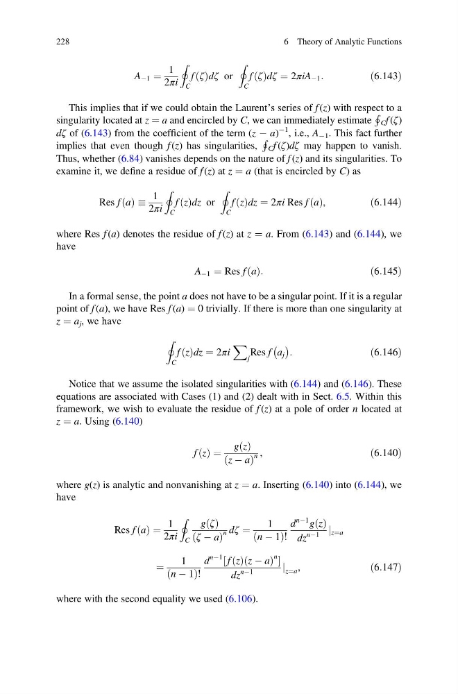
This implies that if we could obtain the Laurent’s series of f (z) with respect to a
singularity located at z ¼ a and encircled by C, we can immediately estimate
H
C f (ζ)
dζ of (6.143) from the coefficient of the term (z À a)
À1 , i.e., A À1 . This fact further
implies that even though f (z) has singularities,
H
C f (ζ)dζ may happen to vanish.
Thus, whether (6.84) vanishes depends on the nature of f (z) and its singularities. To
examine it, we define a residue of f (z) at z ¼ a (that is encircled by C) as
Res f a
ð Þ
1
2πi
I
C
f z
ð Þdz or
I
C
f z
ð Þdz ¼ 2πi Res f a
ð Þ,
ð6:144Þ
where Res f (a) denotes the residue of f (z) at z ¼ a. From (6.143) and (6.144), we
have
A À1 ¼ Res f a
ð Þ:
ð6:145Þ
In a formal sense, the point a does not have to be a singular point. If it is a regular
point of f (a), we have Res f (a) ¼ 0 trivially. If there is more than one singularity at
z ¼ a j , we have
I
C
f z
ð Þdz ¼ 2πi
X
j
Res f a j
À Á :
ð6:146Þ
Notice that we assume the isolated singularities with (6.144) and (6.146). These
equations are associated with Cases (1) and (2) dealt with in Sect. 6.5. Within this
framework, we wish to evaluate the residue of f (z) at a pole of order n located at
z ¼ a. Using (6.140)
f z
ð Þ ¼
g z
ð Þ
z À a
ð
Þ
n ,
ð6:140Þ
where g(z) is analytic and nonvanishing at z ¼ a. Inserting (6.140) into (6.144), we
have
Res f a
ð Þ ¼
1
2πi
I
C
g ζ
ð Þ
ζ À a
ð
Þ
n dζ ¼
1
n À 1
ð
Þ!
d
nÀ1 g z
ð Þ
dz
nÀ1
z¼a
j
¼
1
n À 1
ð
Þ!
d
nÀ1 f z
ð Þ z À a
ð
Þ
n
½
Š
dz
nÀ1
j z¼a ,
ð6:147Þ
where with the second equality we used (6.106).
228
6 Theory of Analytic Functions