

E
2
ð Þ
i ¼ i
h j V j ϕ
1
ð Þ
i i:
ð5:18Þ
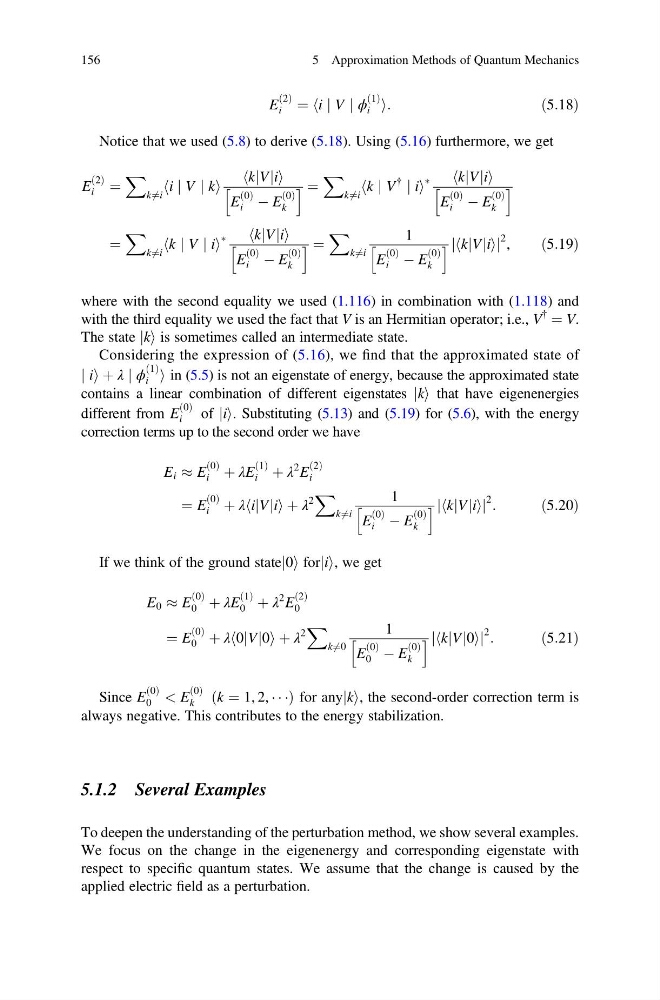
Notice that we used (5.8) to derive (5.18). Using (5.16) furthermore, we get
E
2
ð Þ
i ¼
X
k6 ¼i
i
h j V j ki
kjVji
h
i
E
0
ð Þ
i À E
0
ð Þ
k
h
i¼
X
k6 ¼i
k
h j V
{
j ii
Ã
kjVji
h
i
E
0
ð Þ
i À E
0
ð Þ
k
h
i
¼
X
k6 ¼i
k
h j V j ii
Ã
kjVji
h
i
E
0
ð Þ
i À E
0
ð Þ
k
h
i¼
X
k6 ¼i
1
E
0
ð Þ
i À E
0
ð Þ
k
h
i kjVji
h
i
j
j
2 ,
ð5:19Þ
where with the second equality we used (1.116) in combination with (1.118) and
with the third equality we used the fact that V is an Hermitian operator; i.e., V
{ ¼ V.
The state jki is sometimes called an intermediate state.
Considering the expression of (5.16), we find that the approximated state of
j ii þ λ j ϕ
1
ð Þ
i i in (5.5) is not an eigenstate of energy, because the approximated state
contains a linear combination of different eigenstates jki that have eigenenergies
different from E
0
ð Þ
i
of jii. Substituting (5.13) and (5.19) for (5.6), with the energy
correction terms up to the second order we have
E i % E
0
ð Þ
i þ λE
1
ð Þ
i þ λ
2 E
2
ð Þ
i
¼ E
0
ð Þ
i þ λ ijVji
h
iþ λ
2
X
k6 ¼i
1
E
0
ð Þ
i À E
0
ð Þ
k
h
i kjVji
h
i
j
j
2 :
ð5:20Þ
If we think of the ground statej0i forjii, we get
E 0 % E
0
ð Þ
0 þ λE
1
ð Þ
0 þ λ
2 E
2
ð Þ
0
¼ E
0
ð Þ
0 þ λ 0jVj0
h
iþ λ
2
X
k6 ¼0
1
E
0
ð Þ
0 À E
0
ð Þ
k
h
i kjVj0
h
i
j
j
2 :
ð5:21Þ
Since E
0
ð Þ
0 < E
0
ð Þ
k
k ¼ 1, 2, Á Á Á
ð
Þfor anyjki, the second-order correction term is
always negative. This contributes to the energy stabilization.
5.1.2 Several Examples
To deepen the understanding of the perturbation method, we show several examples.
We focus on the change in the eigenenergy and corresponding eigenstate with
respect to specific quantum states. We assume that the change is caused by the
applied electric field as a perturbation.
156
5 Approximation Methods of Quantum Mechanics
2
ð Þ
i ¼ i
h j V j ϕ
1
ð Þ
i i:
ð5:18Þ
Notice that we used (5.8) to derive (5.18). Using (5.16) furthermore, we get
E
2
ð Þ
i ¼
X
k6 ¼i
i
h j V j ki
kjVji
h
i
E
0
ð Þ
i À E
0
ð Þ
k
h
i¼
X
k6 ¼i
k
h j V
{
j ii
Ã
kjVji
h
i
E
0
ð Þ
i À E
0
ð Þ
k
h
i
¼
X
k6 ¼i
k
h j V j ii
Ã
kjVji
h
i
E
0
ð Þ
i À E
0
ð Þ
k
h
i¼
X
k6 ¼i
1
E
0
ð Þ
i À E
0
ð Þ
k
h
i kjVji
h
i
j
j
2 ,
ð5:19Þ
where with the second equality we used (1.116) in combination with (1.118) and
with the third equality we used the fact that V is an Hermitian operator; i.e., V
{ ¼ V.
The state jki is sometimes called an intermediate state.
Considering the expression of (5.16), we find that the approximated state of
j ii þ λ j ϕ
1
ð Þ
i i in (5.5) is not an eigenstate of energy, because the approximated state
contains a linear combination of different eigenstates jki that have eigenenergies
different from E
0
ð Þ
i
of jii. Substituting (5.13) and (5.19) for (5.6), with the energy
correction terms up to the second order we have
E i % E
0
ð Þ
i þ λE
1
ð Þ
i þ λ
2 E
2
ð Þ
i
¼ E
0
ð Þ
i þ λ ijVji
h
iþ λ
2
X
k6 ¼i
1
E
0
ð Þ
i À E
0
ð Þ
k
h
i kjVji
h
i
j
j
2 :
ð5:20Þ
If we think of the ground statej0i forjii, we get
E 0 % E
0
ð Þ
0 þ λE
1
ð Þ
0 þ λ
2 E
2
ð Þ
0
¼ E
0
ð Þ
0 þ λ 0jVj0
h
iþ λ
2
X
k6 ¼0
1
E
0
ð Þ
0 À E
0
ð Þ
k
h
i kjVj0
h
i
j
j
2 :
ð5:21Þ
Since E
0
ð Þ
0 < E
0
ð Þ
k
k ¼ 1, 2, Á Á Á
ð
Þfor anyjki, the second-order correction term is
always negative. This contributes to the energy stabilization.
5.1.2 Several Examples
To deepen the understanding of the perturbation method, we show several examples.
We focus on the change in the eigenenergy and corresponding eigenstate with
respect to specific quantum states. We assume that the change is caused by the
applied electric field as a perturbation.
156
5 Approximation Methods of Quantum Mechanics