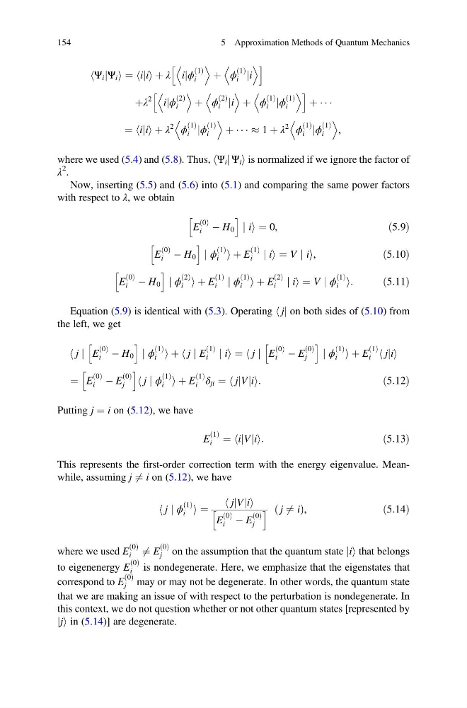
Ψ i jΨ i
h
i¼ iji
h i þ λ ijϕ
1
ð Þ
i
D
E
þ ϕ
1
ð Þ
i ji
D
E
h
i
þλ
2
ijϕ
2
ð Þ
i
D
E
þ ϕ
2
ð Þ
i ji
D
E
þ ϕ
1
ð Þ
i jϕ
1
ð Þ
i
D
E
h
i
þ Á Á Á
¼ iji
h i þ λ
2
ϕ
1
ð Þ
i jϕ
1
ð Þ
i
D
E
þ Á Á Á % 1 þ λ
2
ϕ
1
ð Þ
i jϕ
1
ð Þ
i
D
E
,
where we used (5.4) and (5.8). Thus, hΨ i j Ψ i i is normalized if we ignore the factor of
λ
2 .
Now, inserting (5.5) and (5.6) into (5.1) and comparing the same power factors
with respect to λ, we obtain
E
0
ð Þ
i À H 0
h
i
j ii ¼ 0,
ð5:9Þ
E
0
ð Þ
i À H 0
h
i
j ϕ
1
ð Þ
i i þ E
1
ð Þ
i j ii ¼ V j ii,
ð5:10Þ
E
0
ð Þ
i À H 0
h
i
j ϕ
2
ð Þ
i i þ E
1
ð Þ
i j ϕ
1
ð Þ
i i þ E
2
ð Þ
i j ii ¼ V j ϕ
1
ð Þ
i i:
ð5:11Þ
Equation (5.9) is identical with (5.3). Operating h jj on both sides of (5.10) from
the left, we get
j
h j E
0
ð Þ
i À H 0
h
i
j ϕ
1
ð Þ
i i þ j
h j E
1
ð Þ
i j ii ¼ j
h j E
0
ð Þ
i À E
0
ð Þ
j
h
i
j ϕ
1
ð Þ
i i þ E
1
ð Þ
i
jji
h i
¼ E
0
ð Þ
i À E
0
ð Þ
j
h
i
j
h j ϕ
1
ð Þ
i i þ E
1
ð Þ
i δ ji ¼ jjVji
h
i:
ð5:12Þ
Putting j ¼ i on (5.12), we have
E
1
ð Þ
i ¼ ijVji
h
i:
ð5:13Þ
This represents the first-order correction term with the energy eigenvalue. Meanwhile, assuming j 6 ¼ i on (5.12), we have
j
h j ϕ
1
ð Þ
i i ¼
jjVji
h
i
E
0
ð Þ
i À E
0
ð Þ
j
h
i j 6 ¼ i
ð
Þ,
ð5:14Þ
where we used E
0
ð Þ
i 6 ¼ E
0
ð Þ
j on the assumption that the quantum state jii that belongs
to eigenenergy E
0
ð Þ
i
is nondegenerate. Here, we emphasize that the eigenstates that
correspond to E
0
ð Þ
j may or may not be degenerate. In other words, the quantum state
that we are making an issue of with respect to the perturbation is nondegenerate. In
this context, we do not question whether or not other quantum states [represented by
jji in (5.14)] are degenerate.
154
5 Approximation Methods of Quantum Mechanics