

Z 2π
0
dϕ cos ϕ À ωt
ð
Þ¼0:
This is easily shown by suitable variable transformation.
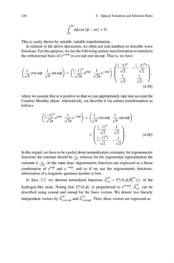
In relation to the above discussion, we often use real numbers to describe wave
functions. For this purpose, we use the following unitary transformation to transform
the orthonormal basis of e
Æimϕ to cos mϕ and sin mϕ. That is, we have
1
ffiffiffi
π
p cos mϕ
1
ffiffiffi
π
p sin mϕ
¼
À1
ð Þ
m
ffiffiffiffiffi
2π
p
e
imϕ
1
ffiffiffiffiffi
2π
p e
Àimϕ
À1
ð Þ
m
ffiffi ffi
2
p
À
À1
ð Þ
m i
ffiffi ffi
2
p
1
ffiffi ffi
2
p
i ffiffi ffi
2
p
0
B
B
@
1
C
C
A ,
ð4:59Þ
where we assume that m is positive so that we can appropriately take into account the
Condon–Shortley phase. Alternatively, we describe it via unitary transformation as
follows:
À1
ð Þ
m
ffiffiffiffiffi
2π
p
e
imϕ
1
ffiffiffiffiffi
2π
p e
Àimϕ
¼
1
ffiffiffi
π
p cos mϕ
1
ffiffiffi
π
p sin mϕ
Â
À1
ð Þ
m
ffiffi ffi
2
p
1
ffiffi ffi
2
p
À1
ð Þ
m i
ffiffi ffi
2
p
À
i ffiffi ffi
2
p
0
B
B
@
1
C
C
A ,
ð4:60Þ
In this regard, we have to be careful about normalization constants; for trigonometric
functions the constant should be
1 ffiffi
π
p , whereas for the exponential representation the
constant is
1 ffiffiffiffi
2π
p . At the same time, trigonometric functions are expressed as a linear
combination of e
imϕ and e
Àimϕ
, and so if we use the trigonometric functions,
information of a magnetic quantum number is lost.
In Sect. 3.7, we showed normalized functions e
Λ
n
ð Þ
l,m ¼ Y
m
l θ, ϕ
ð
Þ e
R
n
ð Þ
l
r
ð Þ of the
hydrogen-like atom. Noting that Y
m
l θ, ϕ
ð
Þ is proportional to e
Æimϕ , e
Λ
n
ð Þ
l,m can be
described using cosmϕ and sinmϕ for the basis vectors. We denote two linearly
independent vectors by e
Λ
n
ð Þ
l, cos mϕ and e
Λ
n
ð Þ
l, sin mϕ . Then, these vectors are expressed as
140
4 Optical Transition and Selection Rules
0
dϕ cos ϕ À ωt
ð
Þ¼0:
This is easily shown by suitable variable transformation.
In relation to the above discussion, we often use real numbers to describe wave
functions. For this purpose, we use the following unitary transformation to transform
the orthonormal basis of e
Æimϕ to cos mϕ and sin mϕ. That is, we have
1
ffiffiffi
π
p cos mϕ
1
ffiffiffi
π
p sin mϕ
¼
À1
ð Þ
m
ffiffiffiffiffi
2π
p
e
imϕ
1
ffiffiffiffiffi
2π
p e
Àimϕ
À1
ð Þ
m
ffiffi ffi
2
p
À
À1
ð Þ
m i
ffiffi ffi
2
p
1
ffiffi ffi
2
p
i ffiffi ffi
2
p
0
B
B
@
1
C
C
A ,
ð4:59Þ
where we assume that m is positive so that we can appropriately take into account the
Condon–Shortley phase. Alternatively, we describe it via unitary transformation as
follows:
À1
ð Þ
m
ffiffiffiffiffi
2π
p
e
imϕ
1
ffiffiffiffiffi
2π
p e
Àimϕ
¼
1
ffiffiffi
π
p cos mϕ
1
ffiffiffi
π
p sin mϕ
Â
À1
ð Þ
m
ffiffi ffi
2
p
1
ffiffi ffi
2
p
À1
ð Þ
m i
ffiffi ffi
2
p
À
i ffiffi ffi
2
p
0
B
B
@
1
C
C
A ,
ð4:60Þ
In this regard, we have to be careful about normalization constants; for trigonometric
functions the constant should be
1 ffiffi
π
p , whereas for the exponential representation the
constant is
1 ffiffiffiffi
2π
p . At the same time, trigonometric functions are expressed as a linear
combination of e
imϕ and e
Àimϕ
, and so if we use the trigonometric functions,
information of a magnetic quantum number is lost.
In Sect. 3.7, we showed normalized functions e
Λ
n
ð Þ
l,m ¼ Y
m
l θ, ϕ
ð
Þ e
R
n
ð Þ
l
r
ð Þ of the
hydrogen-like atom. Noting that Y
m
l θ, ϕ
ð
Þ is proportional to e
Æimϕ , e
Λ
n
ð Þ
l,m can be
described using cosmϕ and sinmϕ for the basis vectors. We denote two linearly
independent vectors by e
Λ
n
ð Þ
l, cos mϕ and e
Λ
n
ð Þ
l, sin mϕ . Then, these vectors are expressed as
140
4 Optical Transition and Selection Rules