

kja ¼
ffiffiffiffiffiffiffiffiffiffiffi
k þ 1
p
k þ 1j
h
D
:
ð4:24Þ
Using (2.62) once again, we get
P kl ¼ e
ffiffiffiffiffiffiffiffiffi ffi
h
2mω
r
ffiffiffiffiffiffiffiffiffiffi ffi
k þ 1
p
k þ 1j
h
li þ
ffiffiffiffiffiffiffiffiffiffi
l þ 1
p
kj
h l þ 1i
h
i
:
ð4:25Þ
Using orthonormal conditions between the state vectors, we have
P kl ¼ e
ffiffiffiffiffiffiffiffiffi ffi
h
2mω
r
ffiffiffiffiffiffiffiffiffiffiffi
k þ 1
p
δ kþ1,l þ
ffiffiffiffiffiffiffiffiffiffi
l þ 1
p
δ k,lþ1
h
i
:
ð4:26Þ
Exchanging k and l in the above, we get
P kl ¼ P lk :
The matrix element P kl is symmetric with respect to indices k and l. Notice that the
first term does not vanish only when k + 1 ¼ l. The second term does not vanish only
when k ¼ l + 1. Therefore we get
P k,kþ1 ¼ e
ffiffiffiffiffiffiffiffiffiffiffiffiffiffiffiffiffi
h k þ 1
ð
Þ
2mω
r
and P lþ1,l ¼ e
ffiffiffiffiffiffiffiffiffiffiffiffiffiffiffiffi
h l þ 1
ð
Þ
2mω
r
or P kþ1,k ¼ e
ffiffiffiffiffiffiffiffiffiffiffiffiffiffiffiffiffi
h k þ 1
ð
Þ
2mω
r
: ð4:27Þ
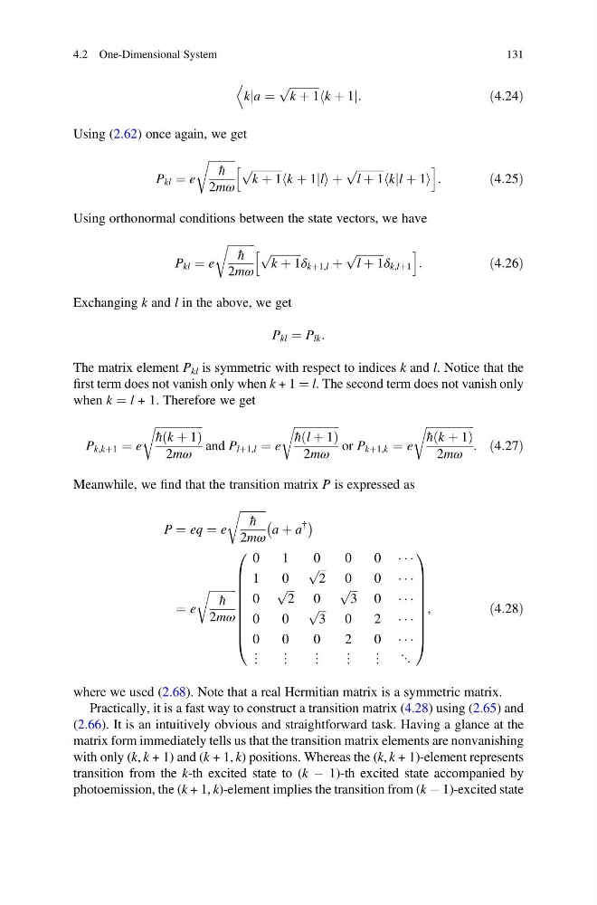
Meanwhile, we find that the transition matrix P is expressed as
P ¼ eq ¼ e
ffiffiffiffiffiffiffiffiffi ffi
h
2mω
r
a þ a
{
À
Á
¼ e
ffiffiffiffiffiffiffiffiffi ffi
h
2mω
r
0
1
0
0
0 Á Á Á
1
0
ffiffi ffi
2
p
0
0 Á Á Á
0
ffiffi ffi
2
p
0
ffiffi ffi
3
p
0 Á Á Á
0
0
ffiffi ffi
3
p
0
2 Á Á Á
0
0
0
2
0 Á Á Á
⋮ ⋮ ⋮ ⋮ ⋮ ⋱
0
B
B
B
B
B
B
B
B
@
1
C
C
C
C
C
C
C
C
A
,
ð4:28Þ
where we used (2.68). Note that a real Hermitian matrix is a symmetric matrix.
Practically, it is a fast way to construct a transition matrix (4.28) using (2.65) and
(2.66). It is an intuitively obvious and straightforward task. Having a glance at the
matrix form immediately tells us that the transition matrix elements are nonvanishing
with only (k, k + 1) and (k + 1, k) positions. Whereas the (k, k + 1)-element represents
transition from the k-th excited state to (k À 1)-th excited state accompanied by
photoemission, the (k + 1, k)-element implies the transition from (k À 1)-excited state
4.2 One-Dimensional System
131
ffiffiffiffiffiffiffiffiffiffiffi
k þ 1
p
k þ 1j
h
D
:
ð4:24Þ
Using (2.62) once again, we get
P kl ¼ e
ffiffiffiffiffiffiffiffiffi ffi
h
2mω
r
ffiffiffiffiffiffiffiffiffiffi ffi
k þ 1
p
k þ 1j
h
li þ
ffiffiffiffiffiffiffiffiffiffi
l þ 1
p
kj
h l þ 1i
h
i
:
ð4:25Þ
Using orthonormal conditions between the state vectors, we have
P kl ¼ e
ffiffiffiffiffiffiffiffiffi ffi
h
2mω
r
ffiffiffiffiffiffiffiffiffiffiffi
k þ 1
p
δ kþ1,l þ
ffiffiffiffiffiffiffiffiffiffi
l þ 1
p
δ k,lþ1
h
i
:
ð4:26Þ
Exchanging k and l in the above, we get
P kl ¼ P lk :
The matrix element P kl is symmetric with respect to indices k and l. Notice that the
first term does not vanish only when k + 1 ¼ l. The second term does not vanish only
when k ¼ l + 1. Therefore we get
P k,kþ1 ¼ e
ffiffiffiffiffiffiffiffiffiffiffiffiffiffiffiffiffi
h k þ 1
ð
Þ
2mω
r
and P lþ1,l ¼ e
ffiffiffiffiffiffiffiffiffiffiffiffiffiffiffiffi
h l þ 1
ð
Þ
2mω
r
or P kþ1,k ¼ e
ffiffiffiffiffiffiffiffiffiffiffiffiffiffiffiffiffi
h k þ 1
ð
Þ
2mω
r
: ð4:27Þ
Meanwhile, we find that the transition matrix P is expressed as
P ¼ eq ¼ e
ffiffiffiffiffiffiffiffiffi ffi
h
2mω
r
a þ a
{
À
Á
¼ e
ffiffiffiffiffiffiffiffiffi ffi
h
2mω
r
0
1
0
0
0 Á Á Á
1
0
ffiffi ffi
2
p
0
0 Á Á Á
0
ffiffi ffi
2
p
0
ffiffi ffi
3
p
0 Á Á Á
0
0
ffiffi ffi
3
p
0
2 Á Á Á
0
0
0
2
0 Á Á Á
⋮ ⋮ ⋮ ⋮ ⋮ ⋱
0
B
B
B
B
B
B
B
B
@
1
C
C
C
C
C
C
C
C
A
,
ð4:28Þ
where we used (2.68). Note that a real Hermitian matrix is a symmetric matrix.
Practically, it is a fast way to construct a transition matrix (4.28) using (2.65) and
(2.66). It is an intuitively obvious and straightforward task. Having a glance at the
matrix form immediately tells us that the transition matrix elements are nonvanishing
with only (k, k + 1) and (k + 1, k) positions. Whereas the (k, k + 1)-element represents
transition from the k-th excited state to (k À 1)-th excited state accompanied by
photoemission, the (k + 1, k)-element implies the transition from (k À 1)-excited state
4.2 One-Dimensional System
131