

Z 0
Àπ=2
ψ
à x, 0
ð Þψ x, 0
ð Þdx ¼
1
2
À
4
3π
% 0:076:
ð4:14Þ
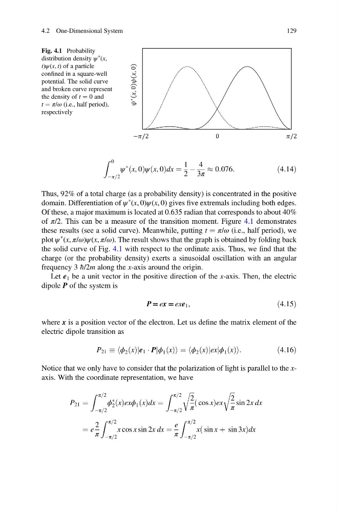
Thus, 92% of a total charge (as a probability density) is concentrated in the positive
domain. Differentiation of ψ
à (x, 0)ψ(x, 0) gives five extremals including both edges.
Of these, a major maximum is located at 0.635 radian that corresponds to about 40%
of π/2. This can be a measure of the transition moment. Figure 4.1 demonstrates
these results (see a solid curve). Meanwhile, putting t ¼ π/ω (i.e., half period), we
plot ψ
à (x, π/ω)ψ(x, π/ω). The result shows that the graph is obtained by folding back
the solid curve of Fig. 4.1 with respect to the ordinate axis. Thus, we find that the
charge (or the probability density) exerts a sinusoidal oscillation with an angular
frequency 3 h/2m along the x-axis around the origin.
Let e 1 be a unit vector in the positive direction of the x-axis. Then, the electric
dipole P of the system is
P = ex = exe 1 ,
ð4:15Þ
where x is a position vector of the electron. Let us define the matrix element of the
electric dipole transition as
P 21 ϕ 2 x
ð Þje 1 Á Pjϕ 1 x
ð Þ
h
i ¼ ϕ 2 x
ð Þjexjϕ 1 x
ð Þ
h
i :
ð4:16Þ
Notice that we only have to consider that the polarization of light is parallel to the xaxis. With the coordinate representation, we have
P 21 ¼
Z π=2
Àπ=2
ϕ
Ã
2 x
ð Þexϕ 1 x
ð Þdx ¼
Z π=2
Àπ=2
ffiffiffi
2
π
r
cos x
ð
Þex
ffiffiffi
2
π
r
sin 2x dx
¼ e
2
π
Z π=2
Àπ=2
x cos x sin 2x dx ¼
e
π
Z π=2
Àπ=2
x sin x þ sin 3x
ð
Þ dx
∗
, 0
, 0
− /2
0
/2
Fig. 4.1 Probability
distribution density ψ
Ã
(x,
t)ψ(x, t) of a particle
confined in a square-well
potential. The solid curve
and broken curve represent
the density of t ¼ 0 and
t ¼ π/ω (i.e., half period),
respectively
4.2 One-Dimensional System
129
Àπ=2
ψ
à x, 0
ð Þψ x, 0
ð Þdx ¼
1
2
À
4
3π
% 0:076:
ð4:14Þ
Thus, 92% of a total charge (as a probability density) is concentrated in the positive
domain. Differentiation of ψ
à (x, 0)ψ(x, 0) gives five extremals including both edges.
Of these, a major maximum is located at 0.635 radian that corresponds to about 40%
of π/2. This can be a measure of the transition moment. Figure 4.1 demonstrates
these results (see a solid curve). Meanwhile, putting t ¼ π/ω (i.e., half period), we
plot ψ
à (x, π/ω)ψ(x, π/ω). The result shows that the graph is obtained by folding back
the solid curve of Fig. 4.1 with respect to the ordinate axis. Thus, we find that the
charge (or the probability density) exerts a sinusoidal oscillation with an angular
frequency 3 h/2m along the x-axis around the origin.
Let e 1 be a unit vector in the positive direction of the x-axis. Then, the electric
dipole P of the system is
P = ex = exe 1 ,
ð4:15Þ
where x is a position vector of the electron. Let us define the matrix element of the
electric dipole transition as
P 21 ϕ 2 x
ð Þje 1 Á Pjϕ 1 x
ð Þ
h
i ¼ ϕ 2 x
ð Þjexjϕ 1 x
ð Þ
h
i :
ð4:16Þ
Notice that we only have to consider that the polarization of light is parallel to the xaxis. With the coordinate representation, we have
P 21 ¼
Z π=2
Àπ=2
ϕ
Ã
2 x
ð Þexϕ 1 x
ð Þdx ¼
Z π=2
Àπ=2
ffiffiffi
2
π
r
cos x
ð
Þex
ffiffiffi
2
π
r
sin 2x dx
¼ e
2
π
Z π=2
Àπ=2
x cos x sin 2x dx ¼
e
π
Z π=2
Àπ=2
x sin x þ sin 3x
ð
Þ dx
∗
, 0
, 0
− /2
0
/2
Fig. 4.1 Probability
distribution density ψ
Ã
(x,
t)ψ(x, t) of a particle
confined in a square-well
potential. The solid curve
and broken curve represent
the density of t ¼ 0 and
t ¼ π/ω (i.e., half period),
respectively
4.2 One-Dimensional System
129