

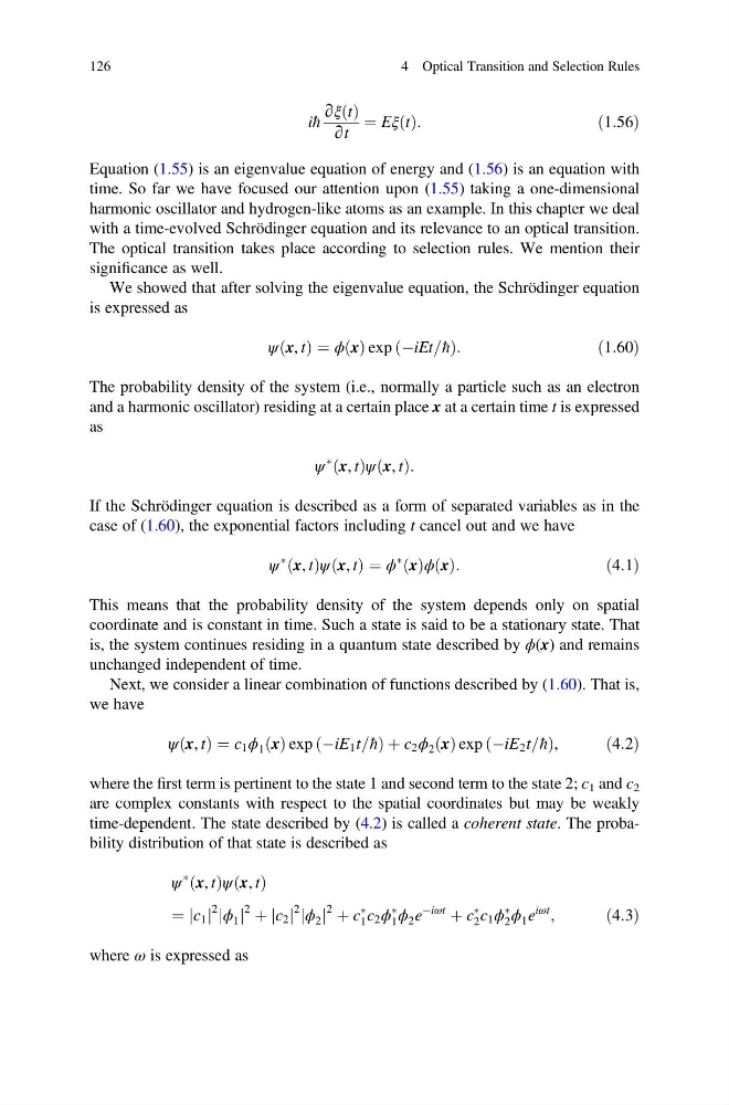
ih
∂ξ t
ð Þ
∂t
¼ Eξ t
ð Þ:
ð1:56Þ
Equation (1.55) is an eigenvalue equation of energy and (1.56) is an equation with
time. So far we have focused our attention upon (1.55) taking a one-dimensional
harmonic oscillator and hydrogen-like atoms as an example. In this chapter we deal
with a time-evolved Schrödinger equation and its relevance to an optical transition.
The optical transition takes place according to selection rules. We mention their
significance as well.
We showed that after solving the eigenvalue equation, the Schrödinger equation
is expressed as
ψ x, t
ð Þ ¼ ϕ x
ð Þ exp ÀiEt=h
ð
Þ :
ð1:60Þ
The probability density of the system (i.e., normally a particle such as an electron
and a harmonic oscillator) residing at a certain place x at a certain time t is expressed
as
ψ
Ã
x, t
ð Þψ x, t
ð Þ:
If the Schrödinger equation is described as a form of separated variables as in the
case of (1.60), the exponential factors including t cancel out and we have
ψ
Ã
x, t
ð Þψ x, t
ð Þ ¼ ϕ
Ã
x
ð Þϕ x
ð Þ:
ð4:1Þ
This means that the probability density of the system depends only on spatial
coordinate and is constant in time. Such a state is said to be a stationary state. That
is, the system continues residing in a quantum state described by ϕ(x) and remains
unchanged independent of time.
Next, we consider a linear combination of functions described by (1.60). That is,
we have
ψ x, t
ð Þ ¼ c 1 ϕ 1 x
ð Þ exp ÀiE 1 t=h
ð
Þþc 2 ϕ 2 x
ð Þ exp ÀiE 2 t=h
ð
Þ ,
ð4:2Þ
where the first term is pertinent to the state 1 and second term to the state 2; c 1 and c 2
are complex constants with respect to the spatial coordinates but may be weakly
time-dependent. The state described by (4.2) is called a coherent state. The probability distribution of that state is described as
ψ
Ã
x, t
ð Þψ x, t
ð Þ
¼ c 1
j j
2 ϕ 1
j j
2 þ c 2
j j
2 ϕ 2
j j
2 þ c
Ã
1 c 2 ϕ
Ã
1 ϕ 2 e
Àiωt
þ c
Ã
2 c 1 ϕ
Ã
2 ϕ 1 e
iωt ,
ð4:3Þ
where ω is expressed as
126
4 Optical Transition and Selection Rules
∂ξ t
ð Þ
∂t
¼ Eξ t
ð Þ:
ð1:56Þ
Equation (1.55) is an eigenvalue equation of energy and (1.56) is an equation with
time. So far we have focused our attention upon (1.55) taking a one-dimensional
harmonic oscillator and hydrogen-like atoms as an example. In this chapter we deal
with a time-evolved Schrödinger equation and its relevance to an optical transition.
The optical transition takes place according to selection rules. We mention their
significance as well.
We showed that after solving the eigenvalue equation, the Schrödinger equation
is expressed as
ψ x, t
ð Þ ¼ ϕ x
ð Þ exp ÀiEt=h
ð
Þ :
ð1:60Þ
The probability density of the system (i.e., normally a particle such as an electron
and a harmonic oscillator) residing at a certain place x at a certain time t is expressed
as
ψ
Ã
x, t
ð Þψ x, t
ð Þ:
If the Schrödinger equation is described as a form of separated variables as in the
case of (1.60), the exponential factors including t cancel out and we have
ψ
Ã
x, t
ð Þψ x, t
ð Þ ¼ ϕ
Ã
x
ð Þϕ x
ð Þ:
ð4:1Þ
This means that the probability density of the system depends only on spatial
coordinate and is constant in time. Such a state is said to be a stationary state. That
is, the system continues residing in a quantum state described by ϕ(x) and remains
unchanged independent of time.
Next, we consider a linear combination of functions described by (1.60). That is,
we have
ψ x, t
ð Þ ¼ c 1 ϕ 1 x
ð Þ exp ÀiE 1 t=h
ð
Þþc 2 ϕ 2 x
ð Þ exp ÀiE 2 t=h
ð
Þ ,
ð4:2Þ
where the first term is pertinent to the state 1 and second term to the state 2; c 1 and c 2
are complex constants with respect to the spatial coordinates but may be weakly
time-dependent. The state described by (4.2) is called a coherent state. The probability distribution of that state is described as
ψ
Ã
x, t
ð Þψ x, t
ð Þ
¼ c 1
j j
2 ϕ 1
j j
2 þ c 2
j j
2 ϕ 2
j j
2 þ c
Ã
1 c 2 ϕ
Ã
1 ϕ 2 e
Àiωt
þ c
Ã
2 c 1 ϕ
Ã
2 ϕ 1 e
iωt ,
ð4:3Þ
where ω is expressed as
126
4 Optical Transition and Selection Rules