

3.1 Introduction
55
Table 3.1 (continued)
Symbol Quantity [unit]
Equations
ν
Vibrational or rotational frequency
(3.24)
ω e
Harmonic vibrational frequency [cm −1 ]
(3.7, 3.9, 3.49)
ω e x e
Anharmonicity constant [cm −1 ]
(3.16, 3.49, 3.50)
ω e y e
Higher-order anharmonicity constant [cm −1 ]
(3.49)
ξ
Expansion parameter for the development of the potential
(3.15)
References books for this section are: Barrow (1962), Brown and Carrington
(2003), Gordy and Cook (1984), Herzberg (1950), Le Roy (2011), and Tiemann
(1992).
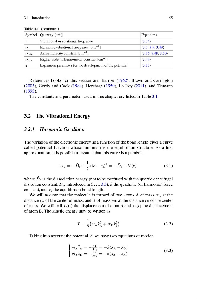
The constants and parameters used in this chapter are listed in Table 3.1.
3.2 The Vibrational Energy
3.2.1 Harmonic Oscillator
The variation of the electronic energy as a function of the bond length gives a curve
called potential function whose minimum is the equilibrium structure. As a first
approximation, it is possible to assume that this curve is a parabola
U V = − ˜
D e +
1
2
k(r − r e )
2
= − ˜
D e + V (r )
(3.1)
where ˜
D e is the dissociation energy (not to be confused with the quartic centrifugal
distortion constant, D e , introduced in Sect. 3.5), k the quadratic (or harmonic) force
constant, and r e the equilibrium bond length.
We will assume that the molecule is formed of two atoms A of mass m A at the
distance r A of the center of mass, and B of mass m B at the distance r B of the center
of mass. We will call x A (t) the displacement of atom A and x B (t) the displacement
of atom B. The kinetic energy may be written as
T =
1
2
m A ˙
x
2
A + m B ˙
x
2
B
(3.2)
Taking into account the potential V, we have two equations of motion
m A ¨
x A = −
∂ V
∂ x A
= −k(x A − x B )
m B ¨
x B = −
∂ V
∂ x B
= −k(x B − x A )
(3.3)
55
Table 3.1 (continued)
Symbol Quantity [unit]
Equations
ν
Vibrational or rotational frequency
(3.24)
ω e
Harmonic vibrational frequency [cm −1 ]
(3.7, 3.9, 3.49)
ω e x e
Anharmonicity constant [cm −1 ]
(3.16, 3.49, 3.50)
ω e y e
Higher-order anharmonicity constant [cm −1 ]
(3.49)
ξ
Expansion parameter for the development of the potential
(3.15)
References books for this section are: Barrow (1962), Brown and Carrington
(2003), Gordy and Cook (1984), Herzberg (1950), Le Roy (2011), and Tiemann
(1992).
The constants and parameters used in this chapter are listed in Table 3.1.
3.2 The Vibrational Energy
3.2.1 Harmonic Oscillator
The variation of the electronic energy as a function of the bond length gives a curve
called potential function whose minimum is the equilibrium structure. As a first
approximation, it is possible to assume that this curve is a parabola
U V = − ˜
D e +
1
2
k(r − r e )
2
= − ˜
D e + V (r )
(3.1)
where ˜
D e is the dissociation energy (not to be confused with the quartic centrifugal
distortion constant, D e , introduced in Sect. 3.5), k the quadratic (or harmonic) force
constant, and r e the equilibrium bond length.
We will assume that the molecule is formed of two atoms A of mass m A at the
distance r A of the center of mass, and B of mass m B at the distance r B of the center
of mass. We will call x A (t) the displacement of atom A and x B (t) the displacement
of atom B. The kinetic energy may be written as
T =
1
2
m A ˙
x
2
A + m B ˙
x
2
B
(3.2)
Taking into account the potential V, we have two equations of motion
m A ¨
x A = −
∂ V
∂ x A
= −k(x A − x B )
m B ¨
x B = −
∂ V
∂ x B
= −k(x B − x A )
(3.3)