

9.10 Systematic Errors
257
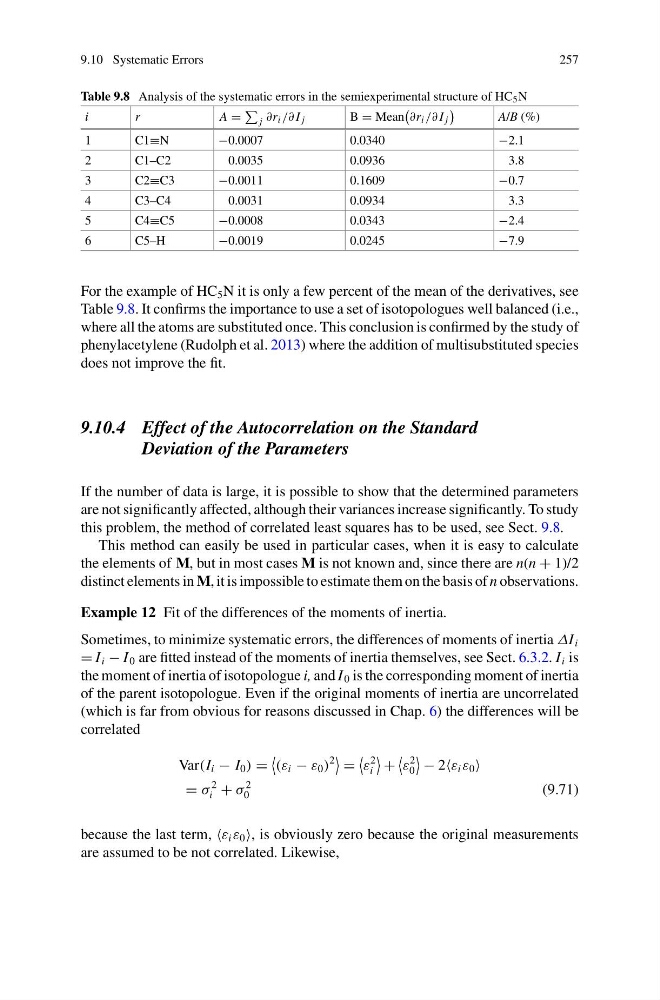
Table 9.8 Analysis of the systematic errors in the semiexperimental structure of HC 5 N
i
r
A =
j ∂r i /∂ I j
B = Mean
∂r i /∂ I j
A/B (%)
1
C1≡N
−0.0007
0.0340
−2.1
2
C1–C2
0.0035
0.0936
3.8
3
C2≡C3
−0.0011
0.1609
−0.7
4
C3–C4
0.0031
0.0934
3.3
5
C4≡C5
−0.0008
0.0343
−2.4
6
C5–H
−0.0019
0.0245
−7.9
For the example of HC 5 N it is only a few percent of the mean of the derivatives, see
Table 9.8. It confirms the importance to use a set of isotopologues well balanced (i.e.,
where all the atoms are substituted once. This conclusion is confirmed by the study of
phenylacetylene (Rudolph et al. 2013) where the addition of multisubstituted species
does not improve the fit.
9.10.4 Effect of the Autocorrelation on the Standard
Deviation of the Parameters
If the number of data is large, it is possible to show that the determined parameters
are not significantly affected, although their variances increase significantly. To study
this problem, the method of correlated least squares has to be used, see Sect. 9.8.
This method can easily be used in particular cases, when it is easy to calculate
the elements of M, but in most cases M is not known and, since there are n(n + 1)/2
distinct elements in M, it is impossible to estimate them on the basis of n observations.
Example 12 Fit of the differences of the moments of inertia.
Sometimes, to minimize systematic errors, the differences of moments of inertia ΔI i
= I i − I 0 are fitted instead of the moments of inertia themselves, see Sect. 6.3.2. I i is
the moment of inertia of isotopologue i, and I 0 is the corresponding moment of inertia
of the parent isotopologue. Even if the original moments of inertia are uncorrelated
(which is far from obvious for reasons discussed in Chap. 6) the differences will be
correlated
Var(I i − I 0 ) =
(ε i − ε 0 )
2
=
ε
2
i
+
ε
2
0
− 2ε i ε 0
= σ
2
i + σ
2
0
(9.71)
because the last term, ε i ε 0 , is obviously zero because the original measurements
are assumed to be not correlated. Likewise,
257
Table 9.8 Analysis of the systematic errors in the semiexperimental structure of HC 5 N
i
r
A =
j ∂r i /∂ I j
B = Mean
∂r i /∂ I j
A/B (%)
1
C1≡N
−0.0007
0.0340
−2.1
2
C1–C2
0.0035
0.0936
3.8
3
C2≡C3
−0.0011
0.1609
−0.7
4
C3–C4
0.0031
0.0934
3.3
5
C4≡C5
−0.0008
0.0343
−2.4
6
C5–H
−0.0019
0.0245
−7.9
For the example of HC 5 N it is only a few percent of the mean of the derivatives, see
Table 9.8. It confirms the importance to use a set of isotopologues well balanced (i.e.,
where all the atoms are substituted once. This conclusion is confirmed by the study of
phenylacetylene (Rudolph et al. 2013) where the addition of multisubstituted species
does not improve the fit.
9.10.4 Effect of the Autocorrelation on the Standard
Deviation of the Parameters
If the number of data is large, it is possible to show that the determined parameters
are not significantly affected, although their variances increase significantly. To study
this problem, the method of correlated least squares has to be used, see Sect. 9.8.
This method can easily be used in particular cases, when it is easy to calculate
the elements of M, but in most cases M is not known and, since there are n(n + 1)/2
distinct elements in M, it is impossible to estimate them on the basis of n observations.
Example 12 Fit of the differences of the moments of inertia.
Sometimes, to minimize systematic errors, the differences of moments of inertia ΔI i
= I i − I 0 are fitted instead of the moments of inertia themselves, see Sect. 6.3.2. I i is
the moment of inertia of isotopologue i, and I 0 is the corresponding moment of inertia
of the parent isotopologue. Even if the original moments of inertia are uncorrelated
(which is far from obvious for reasons discussed in Chap. 6) the differences will be
correlated
Var(I i − I 0 ) =
(ε i − ε 0 )
2
=
ε
2
i
+
ε
2
0
− 2ε i ε 0
= σ
2
i + σ
2
0
(9.71)
because the last term, ε i ε 0 , is obviously zero because the original measurements
are assumed to be not correlated. Likewise,