

9.10 Systematic Errors
255
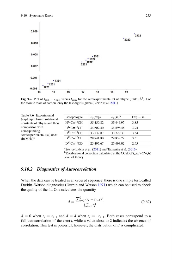
Fig. 9.2 Plot of I exp. − I calc. versus I calc. for the semiexperimental fit of ethyne (unit: uÅ 2 ). For
the atomic mass of carbon, only the last digit is given (Liévin et al. 2011)
Table 9.6 Experimental
(exp) equilibrium rotational
constants of ethyne and their
comparison with
corresponding
semiexperimental (se) ones
(in MHz) a
Isotopologue
B e (exp)
B e (se) b
Exp − se
H 12 C≡ 12 CH
35,450.82
35,446.97
3.85
H 12 C≡ 13 CH
34,602.40
34,598.46
3.94
H 13 C≡ 13 CH
33,732.87
33,729.33
3.54
D 12 C≡ 12 CH
29,841.80
29,838.29
3.51
D 12 C≡ 12 CD
25,495.67
25,493.02
2.65
a Source Liévin et al. (2011) and Tamassia et al. (2016)
b Rovibrational correction calculated at the CCSD(T)_ae/wCVQZ
level of theory
9.10.2 Diagnostics of Autocorrelation
When the data can be treated as an ordered sequence, there is one simple test, called
Durbin–Watson diagnostics (Durbin and Watson 1971) which can be used to check
the quality of the fit. One calculates the quantity
d =
2
i=2 (r i − r i−1 )
2
n
i=1 r
2
i
(9.69)
d = 0 when r i = r i−1 and d = 4 when r i = –r i−1 . Both cases correspond to a
full autocorrelation of the errors, while a value close to 2 indicates the absence of
correlation. This test is powerful; however, the distribution of d is complicated.
255
Fig. 9.2 Plot of I exp. − I calc. versus I calc. for the semiexperimental fit of ethyne (unit: uÅ 2 ). For
the atomic mass of carbon, only the last digit is given (Liévin et al. 2011)
Table 9.6 Experimental
(exp) equilibrium rotational
constants of ethyne and their
comparison with
corresponding
semiexperimental (se) ones
(in MHz) a
Isotopologue
B e (exp)
B e (se) b
Exp − se
H 12 C≡ 12 CH
35,450.82
35,446.97
3.85
H 12 C≡ 13 CH
34,602.40
34,598.46
3.94
H 13 C≡ 13 CH
33,732.87
33,729.33
3.54
D 12 C≡ 12 CH
29,841.80
29,838.29
3.51
D 12 C≡ 12 CD
25,495.67
25,493.02
2.65
a Source Liévin et al. (2011) and Tamassia et al. (2016)
b Rovibrational correction calculated at the CCSD(T)_ae/wCVQZ
level of theory
9.10.2 Diagnostics of Autocorrelation
When the data can be treated as an ordered sequence, there is one simple test, called
Durbin–Watson diagnostics (Durbin and Watson 1971) which can be used to check
the quality of the fit. One calculates the quantity
d =
2
i=2 (r i − r i−1 )
2
n
i=1 r
2
i
(9.69)
d = 0 when r i = r i−1 and d = 4 when r i = –r i−1 . Both cases correspond to a
full autocorrelation of the errors, while a value close to 2 indicates the absence of
correlation. This test is powerful; however, the distribution of d is complicated.