

244
9 Least-Squares Method
Then,
DFBETAS j (i) =
C ji
n
k=1 C
2
jk
r i
s(i)(1 − h ii )
(9.30)
and s(i) is given by
s
2
(i) =
(n − p)s
2
−
r
2
i
1−h ii
n − p − 1
(9.31)
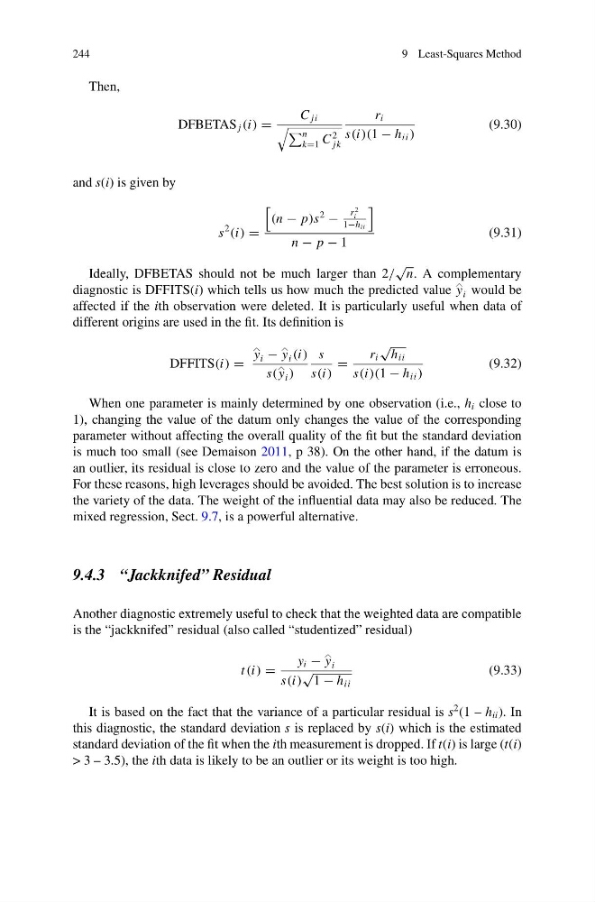
Ideally, DFBETAS should not be much larger than 2/
√
n. A complementary
diagnostic is DFFITS(i) which tells us how much the predicted value y
i would be
affected if the ith observation were deleted. It is particularly useful when data of
different origins are used in the fit. Its definition is
DFFITS(i) =
y
i − y
i (i)
s(y
i )
s
s(i)
=
r i
√
h ii
s(i)(1 − h ii )
(9.32)
When one parameter is mainly determined by one observation (i.e., h i close to
1), changing the value of the datum only changes the value of the corresponding
parameter without affecting the overall quality of the fit but the standard deviation
is much too small (see Demaison 2011, p 38). On the other hand, if the datum is
an outlier, its residual is close to zero and the value of the parameter is erroneous.
For these reasons, high leverages should be avoided. The best solution is to increase
the variety of the data. The weight of the influential data may also be reduced. The
mixed regression, Sect. 9.7, is a powerful alternative.
9.4.3 “Jackknifed” Residual
Another diagnostic extremely useful to check that the weighted data are compatible
is the “jackknifed” residual (also called “studentized” residual)
t (i) =
y i − y
i
s(i)
√
1 − h ii
(9.33)
It is based on the fact that the variance of a particular residual is s
2 (1 – h ii ). In
this diagnostic, the standard deviation s is replaced by s(i) which is the estimated
standard deviation of the fit when the ith measurement is dropped. If t(i) is large (t(i)
> 3 – 3.5), the ith data is likely to be an outlier or its weight is too high.
9 Least-Squares Method
Then,
DFBETAS j (i) =
C ji
n
k=1 C
2
jk
r i
s(i)(1 − h ii )
(9.30)
and s(i) is given by
s
2
(i) =
(n − p)s
2
−
r
2
i
1−h ii
n − p − 1
(9.31)
Ideally, DFBETAS should not be much larger than 2/
√
n. A complementary
diagnostic is DFFITS(i) which tells us how much the predicted value y
i would be
affected if the ith observation were deleted. It is particularly useful when data of
different origins are used in the fit. Its definition is
DFFITS(i) =
y
i − y
i (i)
s(y
i )
s
s(i)
=
r i
√
h ii
s(i)(1 − h ii )
(9.32)
When one parameter is mainly determined by one observation (i.e., h i close to
1), changing the value of the datum only changes the value of the corresponding
parameter without affecting the overall quality of the fit but the standard deviation
is much too small (see Demaison 2011, p 38). On the other hand, if the datum is
an outlier, its residual is close to zero and the value of the parameter is erroneous.
For these reasons, high leverages should be avoided. The best solution is to increase
the variety of the data. The weight of the influential data may also be reduced. The
mixed regression, Sect. 9.7, is a powerful alternative.
9.4.3 “Jackknifed” Residual
Another diagnostic extremely useful to check that the weighted data are compatible
is the “jackknifed” residual (also called “studentized” residual)
t (i) =
y i − y
i
s(i)
√
1 − h ii
(9.33)
It is based on the fact that the variance of a particular residual is s
2 (1 – h ii ). In
this diagnostic, the standard deviation s is replaced by s(i) which is the estimated
standard deviation of the fit when the ith measurement is dropped. If t(i) is large (t(i)
> 3 – 3.5), the ith data is likely to be an outlier or its weight is too high.