

9.4 Diagnostics
241
η k =
μ max
μ k
k = 1, . . . , p
(9.23)
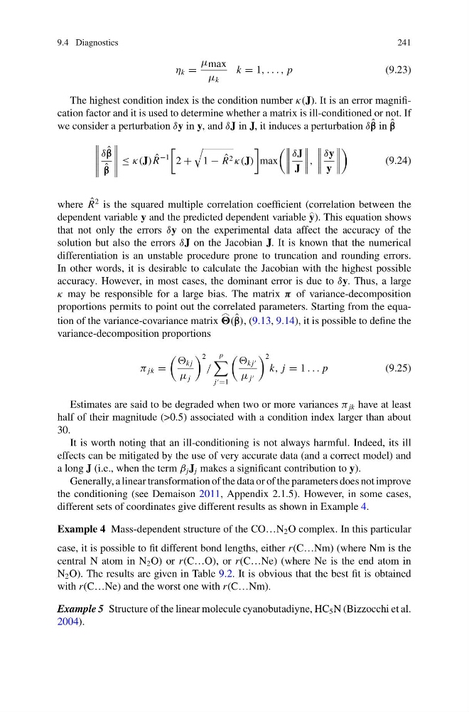
The highest condition index is the condition number κ(J). It is an error magnification factor and it is used to determine whether a matrix is ill-conditioned or not. If
we consider a perturbation δy in y, and δJ in J, it induces a perturbation δ ˆ
β in ˆ
β
δ ˆ
β
ˆ
β
≤ κ(J) ˆ
R
−1
2 +
1 − ˆ
R 2 κ(J)
max
δJ
J
,
δy
y
(9.24)
where ˆ
R
2 is the squared multiple correlation coefficient (correlation between the
dependent variable y and the predicted dependent variable y
). This equation shows
that not only the errors δy on the experimental data affect the accuracy of the
solution but also the errors δJ on the Jacobian J. It is known that the numerical
differentiation is an unstable procedure prone to truncation and rounding errors.
In other words, it is desirable to calculate the Jacobian with the highest possible
accuracy. However, in most cases, the dominant error is due to δy. Thus, a large
κ may be responsible for a large bias. The matrix π of variance-decomposition
proportions permits to point out the correlated parameters. Starting from the equation of the variance-covariance matrix
( ˆ
β), (9.13, 9.14), it is possible to define the
variance-decomposition proportions
π jk =
k j
μ j
2
/
p
j =1
k j
μ j
2
k, j = 1 . . . p
(9.25)
Estimates are said to be degraded when two or more variances π jk have at least
half of their magnitude (>0.5) associated with a condition index larger than about
30.
It is worth noting that an ill-conditioning is not always harmful. Indeed, its ill
effects can be mitigated by the use of very accurate data (and a correct model) and
a long J (i.e., when the term β j J j makes a significant contribution to y).
Generally, a linear transformation of the data or of the parameters does not improve
the conditioning (see Demaison 2011, Appendix 2.1.5). However, in some cases,
different sets of coordinates give different results as shown in Example 4.
Example 4 Mass-dependent structure of the CO…N 2 O complex. In this particular
case, it is possible to fit different bond lengths, either r(C…Nm) (where Nm is the
central N atom in N 2 O) or r(C…O), or r(C…Ne) (where Ne is the end atom in
N 2 O). The results are given in Table 9.2. It is obvious that the best fit is obtained
with r(C…Ne) and the worst one with r(C…Nm).
Example 5 Structure of the linear molecule cyanobutadiyne, HC 5 N (Bizzocchi et al.
2004).
241
η k =
μ max
μ k
k = 1, . . . , p
(9.23)
The highest condition index is the condition number κ(J). It is an error magnification factor and it is used to determine whether a matrix is ill-conditioned or not. If
we consider a perturbation δy in y, and δJ in J, it induces a perturbation δ ˆ
β in ˆ
β
δ ˆ
β
ˆ
β
≤ κ(J) ˆ
R
−1
2 +
1 − ˆ
R 2 κ(J)
max
δJ
J
,
δy
y
(9.24)
where ˆ
R
2 is the squared multiple correlation coefficient (correlation between the
dependent variable y and the predicted dependent variable y
). This equation shows
that not only the errors δy on the experimental data affect the accuracy of the
solution but also the errors δJ on the Jacobian J. It is known that the numerical
differentiation is an unstable procedure prone to truncation and rounding errors.
In other words, it is desirable to calculate the Jacobian with the highest possible
accuracy. However, in most cases, the dominant error is due to δy. Thus, a large
κ may be responsible for a large bias. The matrix π of variance-decomposition
proportions permits to point out the correlated parameters. Starting from the equation of the variance-covariance matrix
( ˆ
β), (9.13, 9.14), it is possible to define the
variance-decomposition proportions
π jk =
k j
μ j
2
/
p
j =1
k j
μ j
2
k, j = 1 . . . p
(9.25)
Estimates are said to be degraded when two or more variances π jk have at least
half of their magnitude (>0.5) associated with a condition index larger than about
30.
It is worth noting that an ill-conditioning is not always harmful. Indeed, its ill
effects can be mitigated by the use of very accurate data (and a correct model) and
a long J (i.e., when the term β j J j makes a significant contribution to y).
Generally, a linear transformation of the data or of the parameters does not improve
the conditioning (see Demaison 2011, Appendix 2.1.5). However, in some cases,
different sets of coordinates give different results as shown in Example 4.
Example 4 Mass-dependent structure of the CO…N 2 O complex. In this particular
case, it is possible to fit different bond lengths, either r(C…Nm) (where Nm is the
central N atom in N 2 O) or r(C…O), or r(C…Ne) (where Ne is the end atom in
N 2 O). The results are given in Table 9.2. It is obvious that the best fit is obtained
with r(C…Ne) and the worst one with r(C…Nm).
Example 5 Structure of the linear molecule cyanobutadiyne, HC 5 N (Bizzocchi et al.
2004).