228
8 Models of Chemical Bonding and “Empirical” Methods
χ i = 1.57
√ χ i
(8.27)
The weak point of this method is that it assigns the same partial charge to each
atom of the same kind. For instance, in CH 3 OH, all the H have the same charge.
Fortunately, Rappé and Goddard (1991) proposed a more sophisticated version.
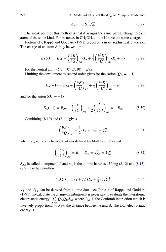
The charge of an atom A may be written
E A (Q) = E A0 +
∂ E
∂ Q
A0
Q A +
1
2
∂
2 E
∂ Q 2
A0
Q
2
A + · · ·
(8.28)
For the neutral atom (Q A = 0): E A (0) = E A0
Limiting the develoment to second order gives for the cation (Q A = + 1)
E A (+1) = E A0 +
∂ E
∂ Q
A0
+
1
2
∂
2 E
∂ Q 2
A0
= E i
(8.29)
and for the anion (Q A = −1)
E A (−1) = E A0 −
∂ E
∂ Q
A0
+
1
2
∂
2 E
∂ Q 2
A0
= −E ca
(8.30)
Combining (8.10) and (8.11) gives
∂ E
∂ Q
A0
=
1
2
(E i + E ca ) = χ
0
A
(8.31)
where χ A is the electronegativity as defined by Mulliken, (8.4) and
∂
2 E
∂ Q 2
A0
= E i − E ca = J
0
AA = 2η
0
A
(8.32)
J AA is called idempotential and η A is the atomic hardness. Using (8.12) and (8.13),
(8.9) may be rewritten
E A (Q) = E A0 + χ
O
A Q A +
1
2
J
0
AA Q
2
A
(8.33)
χ
0
A and J
0
AA can be derived from atomic data, see Table 1 of Rappé and Goddard
(1991). To calculate the charge distribution, it is necessary to evaluate the interatomic
electrostatic energy,
A Q A Q B J AB where J AB is the Coulomb interaction which is
inversely proportional to R AB , the distance between A and B. The total electrostatic
energy is