

6.5 Mass-Dependent Structures
139
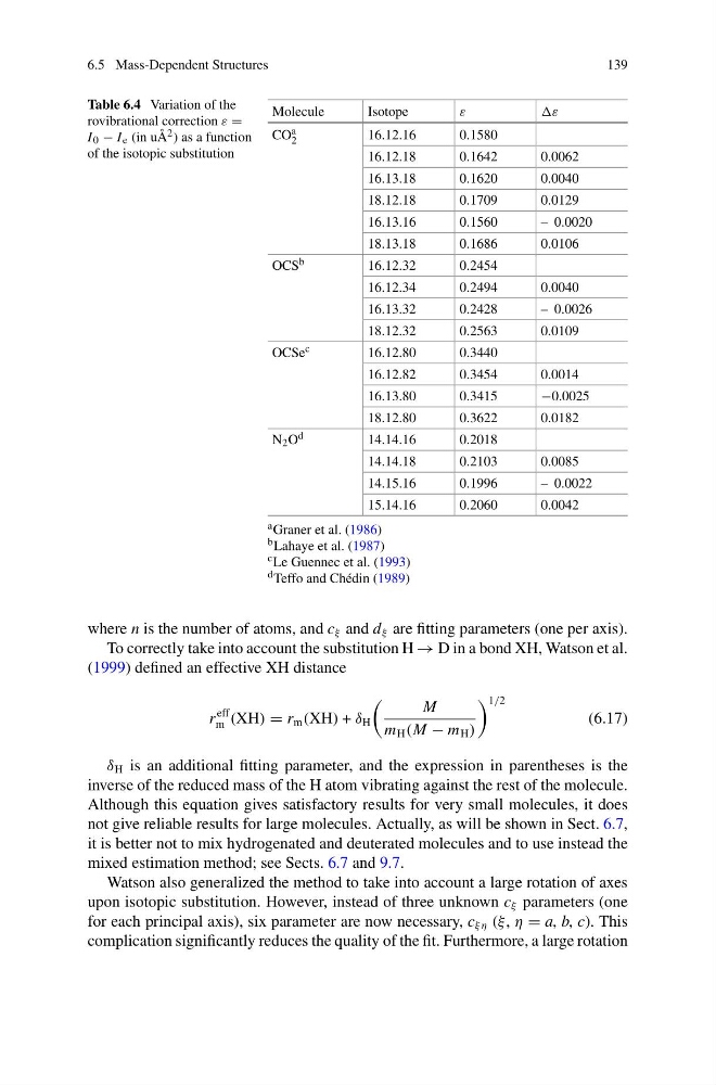
Table 6.4 Variation of the
rovibrational correction ε =
I 0 − I e (in uÅ 2 ) as a function
of the isotopic substitution
Molecule
Isotope
ε
ε
CO a
2
16.12.16
0.1580
16.12.18
0.1642
0.0062
16.13.18
0.1620
0.0040
18.12.18
0.1709
0.0129
16.13.16
0.1560
– 0.0020
18.13.18
0.1686
0.0106
OCS b
16.12.32
0.2454
16.12.34
0.2494
0.0040
16.13.32
0.2428
– 0.0026
18.12.32
0.2563
0.0109
OCSe c
16.12.80
0.3440
16.12.82
0.3454
0.0014
16.13.80
0.3415
−0.0025
18.12.80
0.3622
0.0182
N 2 O d
14.14.16
0.2018
14.14.18
0.2103
0.0085
14.15.16
0.1996
– 0.0022
15.14.16
0.2060
0.0042
a Graner et al. (1986)
b Lahaye et al. (1987)
c Le Guennec et al. (1993)
d Teffo and Chédin (1989)
where n is the number of atoms, and c ξ and d ξ are fitting parameters (one per axis).
To correctly take into account the substitution H → D in a bond XH, Watson et al.
(1999) defined an effective XH distance
r
eff
m (XH) = r m (XH) + δ H
M
m H (M − m H )
1/2
(6.17)
δ H is an additional fitting parameter, and the expression in parentheses is the
inverse of the reduced mass of the H atom vibrating against the rest of the molecule.
Although this equation gives satisfactory results for very small molecules, it does
not give reliable results for large molecules. Actually, as will be shown in Sect. 6.7,
it is better not to mix hydrogenated and deuterated molecules and to use instead the
mixed estimation method; see Sects. 6.7 and 9.7.
Watson also generalized the method to take into account a large rotation of axes
upon isotopic substitution. However, instead of three unknown c ξ parameters (one
for each principal axis), six parameter are now necessary, c ξη (ξ, η = a, b, c). This
complication significantly reduces the quality of the fit. Furthermore, a large rotation
139
Table 6.4 Variation of the
rovibrational correction ε =
I 0 − I e (in uÅ 2 ) as a function
of the isotopic substitution
Molecule
Isotope
ε
ε
CO a
2
16.12.16
0.1580
16.12.18
0.1642
0.0062
16.13.18
0.1620
0.0040
18.12.18
0.1709
0.0129
16.13.16
0.1560
– 0.0020
18.13.18
0.1686
0.0106
OCS b
16.12.32
0.2454
16.12.34
0.2494
0.0040
16.13.32
0.2428
– 0.0026
18.12.32
0.2563
0.0109
OCSe c
16.12.80
0.3440
16.12.82
0.3454
0.0014
16.13.80
0.3415
−0.0025
18.12.80
0.3622
0.0182
N 2 O d
14.14.16
0.2018
14.14.18
0.2103
0.0085
14.15.16
0.1996
– 0.0022
15.14.16
0.2060
0.0042
a Graner et al. (1986)
b Lahaye et al. (1987)
c Le Guennec et al. (1993)
d Teffo and Chédin (1989)
where n is the number of atoms, and c ξ and d ξ are fitting parameters (one per axis).
To correctly take into account the substitution H → D in a bond XH, Watson et al.
(1999) defined an effective XH distance
r
eff
m (XH) = r m (XH) + δ H
M
m H (M − m H )
1/2
(6.17)
δ H is an additional fitting parameter, and the expression in parentheses is the
inverse of the reduced mass of the H atom vibrating against the rest of the molecule.
Although this equation gives satisfactory results for very small molecules, it does
not give reliable results for large molecules. Actually, as will be shown in Sect. 6.7,
it is better not to mix hydrogenated and deuterated molecules and to use instead the
mixed estimation method; see Sects. 6.7 and 9.7.
Watson also generalized the method to take into account a large rotation of axes
upon isotopic substitution. However, instead of three unknown c ξ parameters (one
for each principal axis), six parameter are now necessary, c ξη (ξ, η = a, b, c). This
complication significantly reduces the quality of the fit. Furthermore, a large rotation