

84
J. Fan et al.
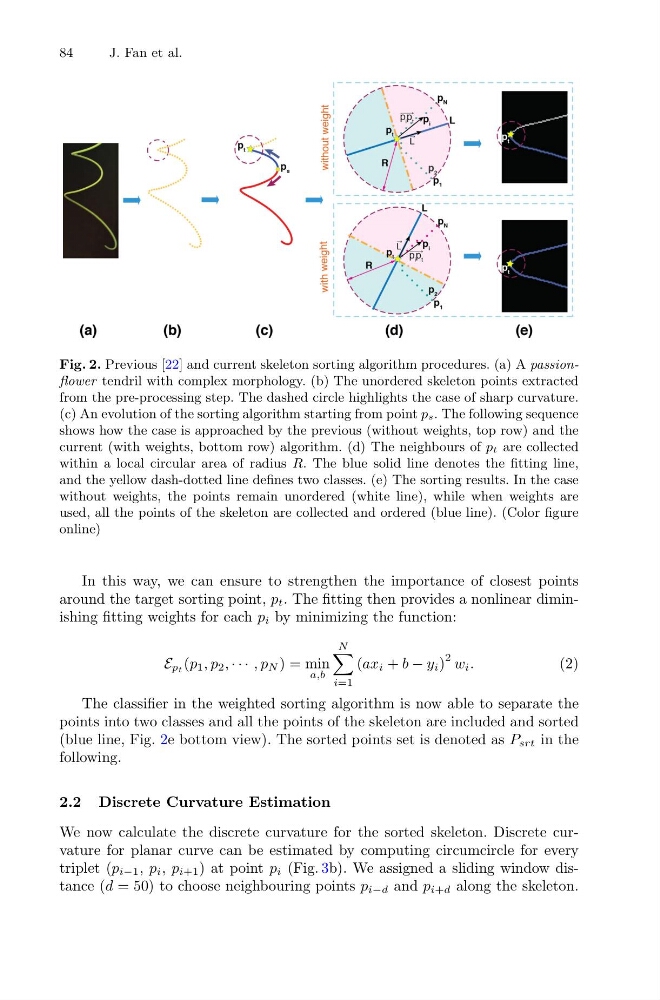
Fig. 2. Previous [22] and current skeleton sorting algorithm procedures. (a) A passionflower tendril with complex morphology. (b) The unordered skeleton points extracted
from the pre-processing step. The dashed circle highlights the case of sharp curvature.
(c) An evolution of the sorting algorithm starting from point ps. The following sequence
shows how the case is approached by the previous (without weights, top row) and the
current (with weights, bottom row) algorithm. (d) The neighbours of pt are collected
within a local circular area of radius R. The blue solid line denotes the fitting line,
and the yellow dash-dotted line defines two classes. (e) The sorting results. In the case
without weights, the points remain unordered (white line), while when weights are
used, all the points of the skeleton are collected and ordered (blue line). (Color figure
online)
In this way, we can ensure to strengthen the importance of closest points
around the target sorting point, p t . The fitting then provides a nonlinear diminishing fitting weights for each p i by minimizing the function:
E pt (p 1 , p 2 , · · · , p N ) = min
a,b
N
i=1
(ax i + b − y i )
2 w i .
(2)
The classifier in the weighted sorting algorithm is now able to separate the
points into two classes and all the points of the skeleton are included and sorted
(blue line, Fig. 2e bottom view). The sorted points set is denoted as P srt in the
following.
2.2 Discrete Curvature Estimation
We now calculate the discrete curvature for the sorted skeleton. Discrete curvature for planar curve can be estimated by computing circumcircle for every
triplet (p i−1 , p i , p i+1 ) at point p i (Fig. 3b). We assigned a sliding window distance (d = 50) to choose neighbouring points p i−d and p i+d along the skeleton.
J. Fan et al.
Fig. 2. Previous [22] and current skeleton sorting algorithm procedures. (a) A passionflower tendril with complex morphology. (b) The unordered skeleton points extracted
from the pre-processing step. The dashed circle highlights the case of sharp curvature.
(c) An evolution of the sorting algorithm starting from point ps. The following sequence
shows how the case is approached by the previous (without weights, top row) and the
current (with weights, bottom row) algorithm. (d) The neighbours of pt are collected
within a local circular area of radius R. The blue solid line denotes the fitting line,
and the yellow dash-dotted line defines two classes. (e) The sorting results. In the case
without weights, the points remain unordered (white line), while when weights are
used, all the points of the skeleton are collected and ordered (blue line). (Color figure
online)
In this way, we can ensure to strengthen the importance of closest points
around the target sorting point, p t . The fitting then provides a nonlinear diminishing fitting weights for each p i by minimizing the function:
E pt (p 1 , p 2 , · · · , p N ) = min
a,b
N
i=1
(ax i + b − y i )
2 w i .
(2)
The classifier in the weighted sorting algorithm is now able to separate the
points into two classes and all the points of the skeleton are included and sorted
(blue line, Fig. 2e bottom view). The sorted points set is denoted as P srt in the
following.
2.2 Discrete Curvature Estimation
We now calculate the discrete curvature for the sorted skeleton. Discrete curvature for planar curve can be estimated by computing circumcircle for every
triplet (p i−1 , p i , p i+1 ) at point p i (Fig. 3b). We assigned a sliding window distance (d = 50) to choose neighbouring points p i−d and p i+d along the skeleton.