

Optimization of Artificial Muscle Placements
263
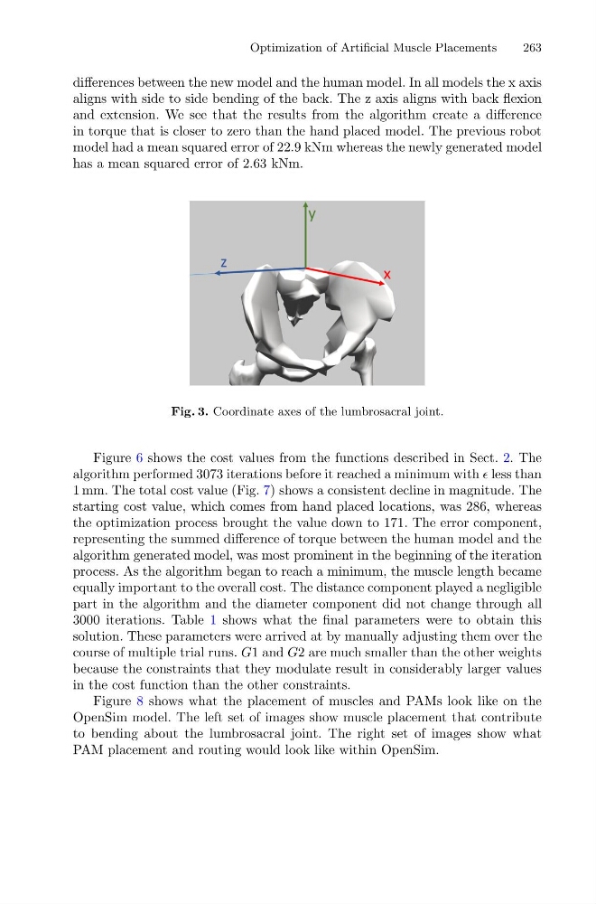
differences between the new model and the human model. In all models the x axis
aligns with side to side bending of the back. The z axis aligns with back flexion
and extension. We see that the results from the algorithm create a difference
in torque that is closer to zero than the hand placed model. The previous robot
model had a mean squared error of 22.9 kNm whereas the newly generated model
has a mean squared error of 2.63 kNm.
Fig. 3. Coordinate axes of the lumbrosacral joint.
Figure 6 shows the cost values from the functions described in Sect. 2. The
algorithm performed 3073 iterations before it reached a minimum with less than
1 mm. The total cost value (Fig. 7) shows a consistent decline in magnitude. The
starting cost value, which comes from hand placed locations, was 286, whereas
the optimization process brought the value down to 171. The error component,
representing the summed difference of torque between the human model and the
algorithm generated model, was most prominent in the beginning of the iteration
process. As the algorithm began to reach a minimum, the muscle length became
equally important to the overall cost. The distance component played a negligible
part in the algorithm and the diameter component did not change through all
3000 iterations. Table 1 shows what the final parameters were to obtain this
solution. These parameters were arrived at by manually adjusting them over the
course of multiple trial runs. G1 and G2 are much smaller than the other weights
because the constraints that they modulate result in considerably larger values
in the cost function than the other constraints.
Figure 8 shows what the placement of muscles and PAMs look like on the
OpenSim model. The left set of images show muscle placement that contribute
to bending about the lumbrosacral joint. The right set of images show what
PAM placement and routing would look like within OpenSim.
263
differences between the new model and the human model. In all models the x axis
aligns with side to side bending of the back. The z axis aligns with back flexion
and extension. We see that the results from the algorithm create a difference
in torque that is closer to zero than the hand placed model. The previous robot
model had a mean squared error of 22.9 kNm whereas the newly generated model
has a mean squared error of 2.63 kNm.
Fig. 3. Coordinate axes of the lumbrosacral joint.
Figure 6 shows the cost values from the functions described in Sect. 2. The
algorithm performed 3073 iterations before it reached a minimum with less than
1 mm. The total cost value (Fig. 7) shows a consistent decline in magnitude. The
starting cost value, which comes from hand placed locations, was 286, whereas
the optimization process brought the value down to 171. The error component,
representing the summed difference of torque between the human model and the
algorithm generated model, was most prominent in the beginning of the iteration
process. As the algorithm began to reach a minimum, the muscle length became
equally important to the overall cost. The distance component played a negligible
part in the algorithm and the diameter component did not change through all
3000 iterations. Table 1 shows what the final parameters were to obtain this
solution. These parameters were arrived at by manually adjusting them over the
course of multiple trial runs. G1 and G2 are much smaller than the other weights
because the constraints that they modulate result in considerably larger values
in the cost function than the other constraints.
Figure 8 shows what the placement of muscles and PAMs look like on the
OpenSim model. The left set of images show muscle placement that contribute
to bending about the lumbrosacral joint. The right set of images show what
PAM placement and routing would look like within OpenSim.