

212
E. Kagioulis et al.
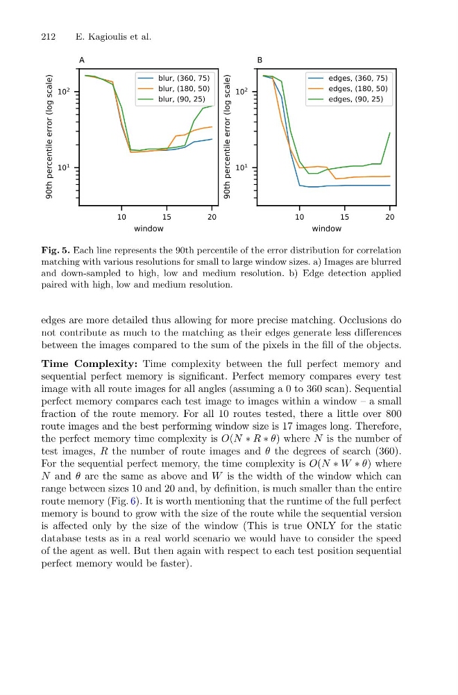
Fig. 5. Each line represents the 90th percentile of the error distribution for correlation
matching with various resolutions for small to large window sizes. a) Images are blurred
and down-sampled to high, low and medium resolution. b) Edge detection applied
paired with high, low and medium resolution.
edges are more detailed thus allowing for more precise matching. Occlusions do
not contribute as much to the matching as their edges generate less differences
between the images compared to the sum of the pixels in the fill of the objects.
Time Complexity: Time complexity between the full perfect memory and
sequential perfect memory is significant. Perfect memory compares every test
image with all route images for all angles (assuming a 0 to 360 scan). Sequential
perfect memory compares each test image to images within a window – a small
fraction of the route memory. For all 10 routes tested, there a little over 800
route images and the best performing window size is 17 images long. Therefore,
the perfect memory time complexity is O(N ∗ R ∗ θ) where N is the number of
test images, R the number of route images and θ the degrees of search (360).
For the sequential perfect memory, the time complexity is O(N ∗ W ∗ θ) where
N and θ are the same as above and W is the width of the window which can
range between sizes 10 and 20 and, by definition, is much smaller than the entire
route memory (Fig. 6). It is worth mentioning that the runtime of the full perfect
memory is bound to grow with the size of the route while the sequential version
is affected only by the size of the window (This is true ONLY for the static
database tests as in a real world scenario we would have to consider the speed
of the agent as well. But then again with respect to each test position sequential
perfect memory would be faster).
E. Kagioulis et al.
Fig. 5. Each line represents the 90th percentile of the error distribution for correlation
matching with various resolutions for small to large window sizes. a) Images are blurred
and down-sampled to high, low and medium resolution. b) Edge detection applied
paired with high, low and medium resolution.
edges are more detailed thus allowing for more precise matching. Occlusions do
not contribute as much to the matching as their edges generate less differences
between the images compared to the sum of the pixels in the fill of the objects.
Time Complexity: Time complexity between the full perfect memory and
sequential perfect memory is significant. Perfect memory compares every test
image with all route images for all angles (assuming a 0 to 360 scan). Sequential
perfect memory compares each test image to images within a window – a small
fraction of the route memory. For all 10 routes tested, there a little over 800
route images and the best performing window size is 17 images long. Therefore,
the perfect memory time complexity is O(N ∗ R ∗ θ) where N is the number of
test images, R the number of route images and θ the degrees of search (360).
For the sequential perfect memory, the time complexity is O(N ∗ W ∗ θ) where
N and θ are the same as above and W is the width of the window which can
range between sizes 10 and 20 and, by definition, is much smaller than the entire
route memory (Fig. 6). It is worth mentioning that the runtime of the full perfect
memory is bound to grow with the size of the route while the sequential version
is affected only by the size of the window (This is true ONLY for the static
database tests as in a real world scenario we would have to consider the speed
of the agent as well. But then again with respect to each test position sequential
perfect memory would be faster).