

A Framework for Resolving Motivational Conflict via Attractor Dynamics
199
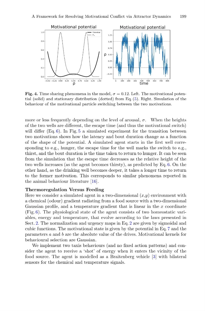
Fig. 4. Time sharing phenomena in the model, σ = 0.12. Left. The motivational potential (solid) and stationary distribution (dotted) from Eq. (5). Right. Simulation of the
behaviour of the motivational particle switching between the two motivations.
more or less frequently depending on the level of arousal, σ. When the heights
of the two wells are different, the escape time (and thus the motivational switch)
will differ (Eq. 6). In Fig. 5 a simulated experiment for the transition between
two motivations shows how the latency and bout duration change as a function
of the shape of the potential. A simulated agent starts in the first well corresponding to e.g., hunger, the escape time for the well marks the switch to e.g.,
thirst, and the bout duration is the time taken to return to hunger. It can be seen
from the simulation that the escape time decreases as the relative height of the
two wells increases (as the agent becomes thirsty), as predicted by Eq. 6. On the
other hand, as the drinking well becomes deeper, it takes a longer time to return
to the former motivation. This corresponds to similar phenomena reported in
the animal behaviour literature [16].
Thermoregulation Versus Feeding
Here we consider a simulated agent in a two-dimensional (x,y) environment with
a chemical (odour) gradient radiating from a food source with a two-dimensional
Gaussian profile, and a temperature gradient that is linear in the x coordinate
(Fig. 6). The physiological state of the agent consists of two homeostatic variables, energy and temperature, that evolve according to the laws presented in
Sect. 2. The normalization and urgency maps in Eq. 2 are given by sigmoidal and
cubic functions. The motivational state is given by the potential in Eq. 7 and the
parameters a and b are the absolute value of the drives. Motivational kernels for
behavioural selection are Gaussian.
We implement two taxis behaviours (and no fixed action patterns) and consider the agent to receive a ‘shot’ of energy when it enters the vicinity of the
food source. The agent is modelled as a Braitenberg vehicle [3] with bilateral
sensors for the chemical and temperature signals.
199
Fig. 4. Time sharing phenomena in the model, σ = 0.12. Left. The motivational potential (solid) and stationary distribution (dotted) from Eq. (5). Right. Simulation of the
behaviour of the motivational particle switching between the two motivations.
more or less frequently depending on the level of arousal, σ. When the heights
of the two wells are different, the escape time (and thus the motivational switch)
will differ (Eq. 6). In Fig. 5 a simulated experiment for the transition between
two motivations shows how the latency and bout duration change as a function
of the shape of the potential. A simulated agent starts in the first well corresponding to e.g., hunger, the escape time for the well marks the switch to e.g.,
thirst, and the bout duration is the time taken to return to hunger. It can be seen
from the simulation that the escape time decreases as the relative height of the
two wells increases (as the agent becomes thirsty), as predicted by Eq. 6. On the
other hand, as the drinking well becomes deeper, it takes a longer time to return
to the former motivation. This corresponds to similar phenomena reported in
the animal behaviour literature [16].
Thermoregulation Versus Feeding
Here we consider a simulated agent in a two-dimensional (x,y) environment with
a chemical (odour) gradient radiating from a food source with a two-dimensional
Gaussian profile, and a temperature gradient that is linear in the x coordinate
(Fig. 6). The physiological state of the agent consists of two homeostatic variables, energy and temperature, that evolve according to the laws presented in
Sect. 2. The normalization and urgency maps in Eq. 2 are given by sigmoidal and
cubic functions. The motivational state is given by the potential in Eq. 7 and the
parameters a and b are the absolute value of the drives. Motivational kernels for
behavioural selection are Gaussian.
We implement two taxis behaviours (and no fixed action patterns) and consider the agent to receive a ‘shot’ of energy when it enters the vicinity of the
food source. The agent is modelled as a Braitenberg vehicle [3] with bilateral
sensors for the chemical and temperature signals.