

A Framework for Resolving Motivational Conflict via Attractor Dynamics
195
More precisely, if ρ(t) represents the position of the particle in the motivational
coordinate, its time evolution is given by
˙
ρ = −
1
τ
∂V
∂ρ
+ σdW (t).
(3)
The first term in the right, V (ρ, a m ), is a potential field that depends upon the
drives, and other motivational factors described shortly, and τ is the time constant for the evolution. We formalize the concept of a motivation by restricting
V : P × R
n
→ R to be a motivational potential if and only if there exist elements ¯
ρ 1 , ¯
ρ 2 , . . . , ¯
ρ k , k > 0 such that
∂V
∂ρ (ρ k , a 1 , . . . , a k ) = 0 when a m = 0 for all
m = 1, . . . , k. This characterizes the initial, undisturbed shape with k motivations. The second term to the right in Eq. 3 is a noise term with variance, σ
2 . We
refer to the variance of the fluctuations, analogous to the influence of heat on
Brownian motion, as arousal. Note that when σ = 0,
dV
dt =
∂V
∂ρ
dρ
dt = −
∂V
∂ρ
2
< 0.
Therefore the dynamics will always tend to select one motivation. Accordingly,
the motivational conflict problem is recast in terms of the escape or Kramers
problems that are familiar in classical statistical mechanics [5]. For fixed drives
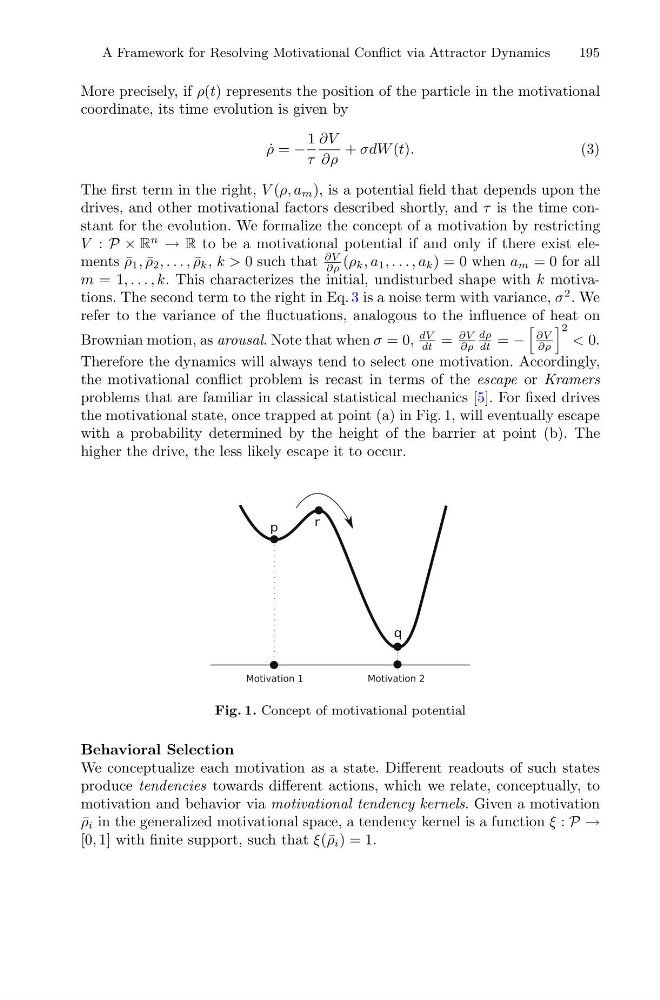
the motivational state, once trapped at point (a) in Fig. 1, will eventually escape
with a probability determined by the height of the barrier at point (b). The
higher the drive, the less likely escape it to occur.
Fig. 1. Concept of motivational potential
Behavioral Selection
We conceptualize each motivation as a state. Different readouts of such states
produce tendencies towards different actions, which we relate, conceptually, to
motivation and behavior via motivational tendency kernels. Given a motivation
¯
ρ i in the generalized motivational space, a tendency kernel is a function ξ : P →
[0, 1] with finite support, such that ξ(¯ ρ i ) = 1.
195
More precisely, if ρ(t) represents the position of the particle in the motivational
coordinate, its time evolution is given by
˙
ρ = −
1
τ
∂V
∂ρ
+ σdW (t).
(3)
The first term in the right, V (ρ, a m ), is a potential field that depends upon the
drives, and other motivational factors described shortly, and τ is the time constant for the evolution. We formalize the concept of a motivation by restricting
V : P × R
n
→ R to be a motivational potential if and only if there exist elements ¯
ρ 1 , ¯
ρ 2 , . . . , ¯
ρ k , k > 0 such that
∂V
∂ρ (ρ k , a 1 , . . . , a k ) = 0 when a m = 0 for all
m = 1, . . . , k. This characterizes the initial, undisturbed shape with k motivations. The second term to the right in Eq. 3 is a noise term with variance, σ
2 . We
refer to the variance of the fluctuations, analogous to the influence of heat on
Brownian motion, as arousal. Note that when σ = 0,
dV
dt =
∂V
∂ρ
dρ
dt = −
∂V
∂ρ
2
< 0.
Therefore the dynamics will always tend to select one motivation. Accordingly,
the motivational conflict problem is recast in terms of the escape or Kramers
problems that are familiar in classical statistical mechanics [5]. For fixed drives
the motivational state, once trapped at point (a) in Fig. 1, will eventually escape
with a probability determined by the height of the barrier at point (b). The
higher the drive, the less likely escape it to occur.
Fig. 1. Concept of motivational potential
Behavioral Selection
We conceptualize each motivation as a state. Different readouts of such states
produce tendencies towards different actions, which we relate, conceptually, to
motivation and behavior via motivational tendency kernels. Given a motivation
¯
ρ i in the generalized motivational space, a tendency kernel is a function ξ : P →
[0, 1] with finite support, such that ξ(¯ ρ i ) = 1.