

From Models of Cognition to Robot Control and Back Using SNNs
181
rotational axes. First of all, u, u x , u adapt , and ˙
q all need to be changed from 2D
to 3D, either due to the increase in number of joints, or increase in number of
cartesian dimensions.
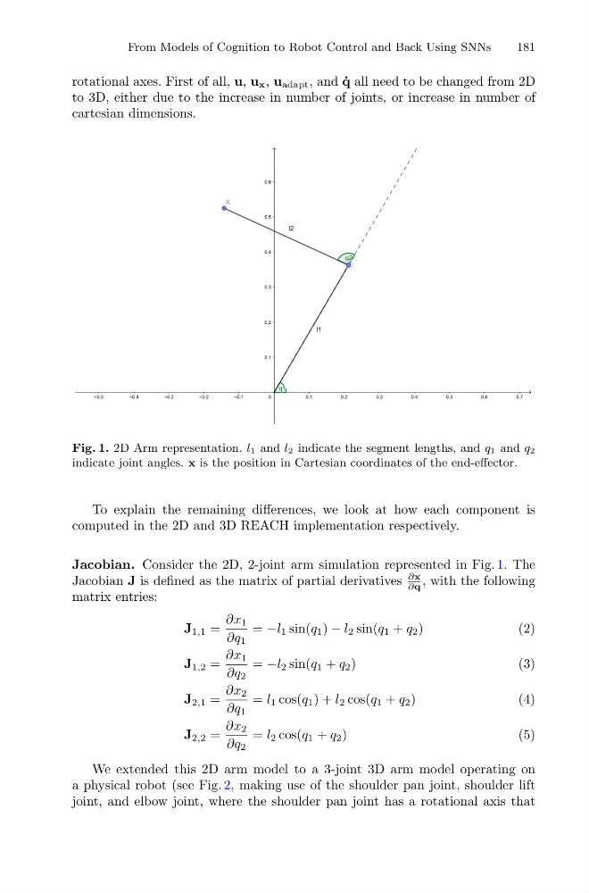
Fig. 1. 2D Arm representation. l1 and l2 indicate the segment lengths, and q1 and q2
indicate joint angles. x is the position in Cartesian coordinates of the end-effector.
To explain the remaining differences, we look at how each component is
computed in the 2D and 3D REACH implementation respectively.
Jacobian. Consider the 2D, 2-joint arm simulation represented in Fig. 1. The
Jacobian J is defined as the matrix of partial derivatives
∂x
∂q , with the following
matrix entries:
J 1,1 =
∂x 1
∂q 1
= −l 1 sin(q 1 ) − l 2 sin(q 1 + q 2 )
(2)
J 1,2 =
∂x 1
∂q 2
= −l 2 sin(q 1 + q 2 )
(3)
J 2,1 =
∂x 2
∂q 1
= l 1 cos(q 1 ) + l 2 cos(q 1 + q 2 )
(4)
J 2,2 =
∂x 2
∂q 2
= l 2 cos(q 1 + q 2 )
(5)
We extended this 2D arm model to a 3-joint 3D arm model operating on
a physical robot (see Fig. 2, making use of the shoulder pan joint, shoulder lift
joint, and elbow joint, where the shoulder pan joint has a rotational axis that
181
rotational axes. First of all, u, u x , u adapt , and ˙
q all need to be changed from 2D
to 3D, either due to the increase in number of joints, or increase in number of
cartesian dimensions.
Fig. 1. 2D Arm representation. l1 and l2 indicate the segment lengths, and q1 and q2
indicate joint angles. x is the position in Cartesian coordinates of the end-effector.
To explain the remaining differences, we look at how each component is
computed in the 2D and 3D REACH implementation respectively.
Jacobian. Consider the 2D, 2-joint arm simulation represented in Fig. 1. The
Jacobian J is defined as the matrix of partial derivatives
∂x
∂q , with the following
matrix entries:
J 1,1 =
∂x 1
∂q 1
= −l 1 sin(q 1 ) − l 2 sin(q 1 + q 2 )
(2)
J 1,2 =
∂x 1
∂q 2
= −l 2 sin(q 1 + q 2 )
(3)
J 2,1 =
∂x 2
∂q 1
= l 1 cos(q 1 ) + l 2 cos(q 1 + q 2 )
(4)
J 2,2 =
∂x 2
∂q 2
= l 2 cos(q 1 + q 2 )
(5)
We extended this 2D arm model to a 3-joint 3D arm model operating on
a physical robot (see Fig. 2, making use of the shoulder pan joint, shoulder lift
joint, and elbow joint, where the shoulder pan joint has a rotational axis that