

136
V. Gabler et al.
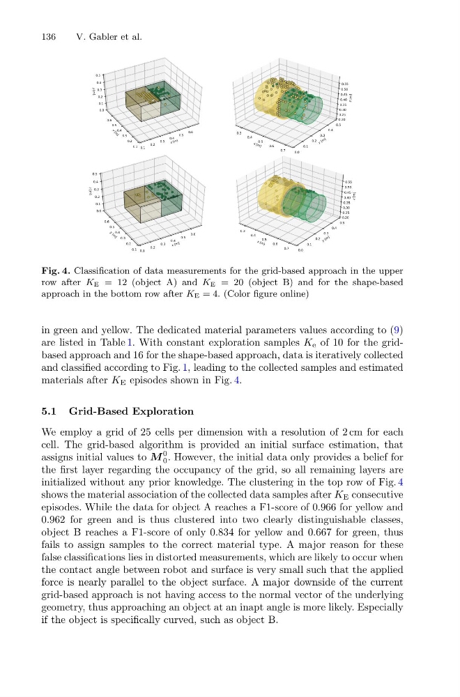
Fig. 4. Classification of data measurements for the grid-based approach in the upper
row after KE = 12 (object A) and KE = 20 (object B) and for the shape-based
approach in the bottom row after KE = 4. (Color figure online)
in green and yellow. The dedicated material parameters values according to (9)
are listed in Table 1. With constant exploration samples K e of 10 for the gridbased approach and 16 for the shape-based approach, data is iteratively collected
and classified according to Fig. 1, leading to the collected samples and estimated
materials after K E episodes shown in Fig. 4.
5.1 Grid-Based Exploration
We employ a grid of 25 cells per dimension with a resolution of 2 cm for each
cell. The grid-based algorithm is provided an initial surface estimation, that
assigns initial values to M
0
0 . However, the initial data only provides a belief for
the first layer regarding the occupancy of the grid, so all remaining layers are
initialized without any prior knowledge. The clustering in the top row of Fig. 4
shows the material association of the collected data samples after K E consecutive
episodes. While the data for object A reaches a F1-score of 0.966 for yellow and
0.962 for green and is thus clustered into two clearly distinguishable classes,
object B reaches a F1-score of only 0.834 for yellow and 0.667 for green, thus
fails to assign samples to the correct material type. A major reason for these
false classifications lies in distorted measurements, which are likely to occur when
the contact angle between robot and surface is very small such that the applied
force is nearly parallel to the object surface. A major downside of the current
grid-based approach is not having access to the normal vector of the underlying
geometry, thus approaching an object at an inapt angle is more likely. Especially
if the object is specifically curved, such as object B.
V. Gabler et al.
Fig. 4. Classification of data measurements for the grid-based approach in the upper
row after KE = 12 (object A) and KE = 20 (object B) and for the shape-based
approach in the bottom row after KE = 4. (Color figure online)
in green and yellow. The dedicated material parameters values according to (9)
are listed in Table 1. With constant exploration samples K e of 10 for the gridbased approach and 16 for the shape-based approach, data is iteratively collected
and classified according to Fig. 1, leading to the collected samples and estimated
materials after K E episodes shown in Fig. 4.
5.1 Grid-Based Exploration
We employ a grid of 25 cells per dimension with a resolution of 2 cm for each
cell. The grid-based algorithm is provided an initial surface estimation, that
assigns initial values to M
0
0 . However, the initial data only provides a belief for
the first layer regarding the occupancy of the grid, so all remaining layers are
initialized without any prior knowledge. The clustering in the top row of Fig. 4
shows the material association of the collected data samples after K E consecutive
episodes. While the data for object A reaches a F1-score of 0.966 for yellow and
0.962 for green and is thus clustered into two clearly distinguishable classes,
object B reaches a F1-score of only 0.834 for yellow and 0.667 for green, thus
fails to assign samples to the correct material type. A major reason for these
false classifications lies in distorted measurements, which are likely to occur when
the contact angle between robot and surface is very small such that the applied
force is nearly parallel to the object surface. A major downside of the current
grid-based approach is not having access to the normal vector of the underlying
geometry, thus approaching an object at an inapt angle is more likely. Especially
if the object is specifically curved, such as object B.