

132
V. Gabler et al.
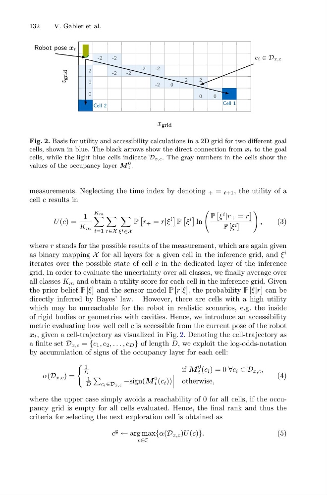
Fig. 2. Basis for utility and accessibility calculations in a 2D grid for two different goal
cells, shown in blue. The black arrows show the direct connection from xt to the goal
cells, while the light blue cells indicate Dx,c. The gray numbers in the cells show the
values of the occupancy layer M
0
t .
measurements. Neglecting the time index by denoting + = t+1 , the utility of a
cell c results in
U (c) =
1
K m
Km
i=1
r∈X
ξ i ∈X
P
r + = r|ξ
i
P
ξ
i
ln
P
ξ
i
|r + = r
P [ξ i ]
,
(3)
where r stands for the possible results of the measurement, which are again given
as binary mapping X for all layers for a given cell in the inference grid, and ξ
i
iterates over the possible state of cell c in the dedicated layer of the inference
grid. In order to evaluate the uncertainty over all classes, we finally average over
all classes K m and obtain a utility score for each cell in the inference grid. Given
the prior belief P [ξ] and the sensor model P [r|ξ], the probability P [ξ|r] can be
directly inferred by Bayes’ law. However, there are cells with a high utility
which may be unreachable for the robot in realistic scenarios, e.g. the inside
of rigid bodies or geometries with cavities. Hence, we introduce an accessibility
metric evaluating how well cell c is accessible from the current pose of the robot
x t , given a cell-trajectory as visualized in Fig. 2. Denoting the cell-trajectory as
a finite set D x,c = {c 1 , c 2 , . . . , c D } of length D, we exploit the log-odds-notation
by accumulation of signs of the occupancy layer for each cell:
α(D x,c ) =
1
D
if M
0
t (c i ) = 0 ∀c i ∈ D x,c ,
1
D
ci∈Dx,c −sign(M
0
t (c i ))
otherwise,
(4)
where the upper case simply avoids a reachability of 0 for all cells, if the occupancy grid is empty for all cells evaluated. Hence, the final rank and thus the
criteria for selecting the next exploration cell is obtained as
c
g
← arg max
c∈C
{α(D x,c )U (c)}.
(5)
V. Gabler et al.
Fig. 2. Basis for utility and accessibility calculations in a 2D grid for two different goal
cells, shown in blue. The black arrows show the direct connection from xt to the goal
cells, while the light blue cells indicate Dx,c. The gray numbers in the cells show the
values of the occupancy layer M
0
t .
measurements. Neglecting the time index by denoting + = t+1 , the utility of a
cell c results in
U (c) =
1
K m
Km
i=1
r∈X
ξ i ∈X
P
r + = r|ξ
i
P
ξ
i
ln
P
ξ
i
|r + = r
P [ξ i ]
,
(3)
where r stands for the possible results of the measurement, which are again given
as binary mapping X for all layers for a given cell in the inference grid, and ξ
i
iterates over the possible state of cell c in the dedicated layer of the inference
grid. In order to evaluate the uncertainty over all classes, we finally average over
all classes K m and obtain a utility score for each cell in the inference grid. Given
the prior belief P [ξ] and the sensor model P [r|ξ], the probability P [ξ|r] can be
directly inferred by Bayes’ law. However, there are cells with a high utility
which may be unreachable for the robot in realistic scenarios, e.g. the inside
of rigid bodies or geometries with cavities. Hence, we introduce an accessibility
metric evaluating how well cell c is accessible from the current pose of the robot
x t , given a cell-trajectory as visualized in Fig. 2. Denoting the cell-trajectory as
a finite set D x,c = {c 1 , c 2 , . . . , c D } of length D, we exploit the log-odds-notation
by accumulation of signs of the occupancy layer for each cell:
α(D x,c ) =
1
D
if M
0
t (c i ) = 0 ∀c i ∈ D x,c ,
1
D
ci∈Dx,c −sign(M
0
t (c i ))
otherwise,
(4)
where the upper case simply avoids a reachability of 0 for all cells, if the occupancy grid is empty for all cells evaluated. Hence, the final rank and thus the
criteria for selecting the next exploration cell is obtained as
c
g
← arg max
c∈C
{α(D x,c )U (c)}.
(5)