

16 Theoretical Foundations of Super-Resolution in Microspherical Nanoscopy
417
0.8
1
1.2
1.4
1.6
1.8
2
2.2
2.4
0
0.5
1
1.5
(a)
(b)
(c)
(d)
P/P
0
D/λ
D/λ=3.5
6.735
6.85
9.8
-9
-6
-3
0
3
6
-6 -3 0 3 6
x/λ
y/λ
y/λ
0
25
50
D/λ=6.735
-9
-6
-3
0
3
6
-6 -3 0 3 6
x/λ
0
5
10
D/λ=6.85
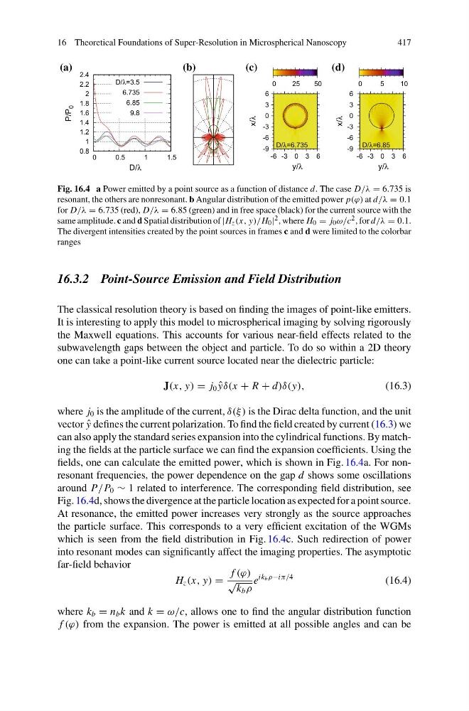
Fig. 16.4 a Power emitted by a point source as a function of distance d. The case D/λ = 6.735 is
resonant, the others are nonresonant. b Angular distribution of the emitted power p(ϕ) at d/λ = 0.1
for D/λ = 6.735 (red), D/λ = 6.85 (green) and in free space (black) for the current source with the
same amplitude. c and d Spatial distribution of |H z (x, y)/H 0 | 2 , where H 0 = j 0 ω/c 2 , for d/λ = 0.1.
The divergent intensities created by the point sources in frames c and d were limited to the colorbar
ranges
16.3.2 Point-Source Emission and Field Distribution
The classical resolution theory is based on finding the images of point-like emitters.
It is interesting to apply this model to microspherical imaging by solving rigorously
the Maxwell equations. This accounts for various near-field effects related to the
subwavelength gaps between the object and particle. To do so within a 2D theory
one can take a point-like current source located near the dielectric particle:
J(x, y) = j 0 ˆ
yδ(x + R + d)δ(y),
(16.3)
where j 0 is the amplitude of the current, δ(ξ ) is the Dirac delta function, and the unit
vector ˆ
y defines the current polarization. To find the field created by current (16.3) we
can also apply the standard series expansion into the cylindrical functions. By matching the fields at the particle surface we can find the expansion coefficients. Using the
fields, one can calculate the emitted power, which is shown in Fig. 16.4a. For nonresonant frequencies, the power dependence on the gap d shows some oscillations
around P/P 0 ∼ 1 related to interference. The corresponding field distribution, see
Fig. 16.4d, shows the divergence at the particle location as expected for a point source.
At resonance, the emitted power increases very strongly as the source approaches
the particle surface. This corresponds to a very efficient excitation of the WGMs
which is seen from the field distribution in Fig. 16.4c. Such redirection of power
into resonant modes can significantly affect the imaging properties. The asymptotic
far-field behavior
H z (x, y) =
f (ϕ)
√
k b ρ
e
ik b ρ−iπ/4
(16.4)
where k b = n b k and k = ω/c, allows one to find the angular distribution function
f (ϕ) from the expansion. The power is emitted at all possible angles and can be
417
0.8
1
1.2
1.4
1.6
1.8
2
2.2
2.4
0
0.5
1
1.5
(a)
(b)
(c)
(d)
P/P
0
D/λ
D/λ=3.5
6.735
6.85
9.8
-9
-6
-3
0
3
6
-6 -3 0 3 6
x/λ
y/λ
y/λ
0
25
50
D/λ=6.735
-9
-6
-3
0
3
6
-6 -3 0 3 6
x/λ
0
5
10
D/λ=6.85
Fig. 16.4 a Power emitted by a point source as a function of distance d. The case D/λ = 6.735 is
resonant, the others are nonresonant. b Angular distribution of the emitted power p(ϕ) at d/λ = 0.1
for D/λ = 6.735 (red), D/λ = 6.85 (green) and in free space (black) for the current source with the
same amplitude. c and d Spatial distribution of |H z (x, y)/H 0 | 2 , where H 0 = j 0 ω/c 2 , for d/λ = 0.1.
The divergent intensities created by the point sources in frames c and d were limited to the colorbar
ranges
16.3.2 Point-Source Emission and Field Distribution
The classical resolution theory is based on finding the images of point-like emitters.
It is interesting to apply this model to microspherical imaging by solving rigorously
the Maxwell equations. This accounts for various near-field effects related to the
subwavelength gaps between the object and particle. To do so within a 2D theory
one can take a point-like current source located near the dielectric particle:
J(x, y) = j 0 ˆ
yδ(x + R + d)δ(y),
(16.3)
where j 0 is the amplitude of the current, δ(ξ ) is the Dirac delta function, and the unit
vector ˆ
y defines the current polarization. To find the field created by current (16.3) we
can also apply the standard series expansion into the cylindrical functions. By matching the fields at the particle surface we can find the expansion coefficients. Using the
fields, one can calculate the emitted power, which is shown in Fig. 16.4a. For nonresonant frequencies, the power dependence on the gap d shows some oscillations
around P/P 0 ∼ 1 related to interference. The corresponding field distribution, see
Fig. 16.4d, shows the divergence at the particle location as expected for a point source.
At resonance, the emitted power increases very strongly as the source approaches
the particle surface. This corresponds to a very efficient excitation of the WGMs
which is seen from the field distribution in Fig. 16.4c. Such redirection of power
into resonant modes can significantly affect the imaging properties. The asymptotic
far-field behavior
H z (x, y) =
f (ϕ)
√
k b ρ
e
ik b ρ−iπ/4
(16.4)
where k b = n b k and k = ω/c, allows one to find the angular distribution function
f (ϕ) from the expansion. The power is emitted at all possible angles and can be