

11 Label-Free Super-Resolution Microscopy by Nonlinear …
283
WF. At modulation frequencies higher than 1000 Hz, the dynamic response of the
AOM differs from the static response. Consequently, after the first stage, the harmonic
content in our setup amounts to 1–2% and corrections to the initial fitting are needed.
In the second stage, that reduces the distortion by about additional two orders of
magnitude, we use an iterative proportional–integral–derivative (PID) control. As in
the first stage, the WF is synthesized by N discrete points defining a single cycle
which is repeated at f m . We assume that the errors at a definite time of the light
intensity are solely determined by a corresponding point in the WF. At each PID
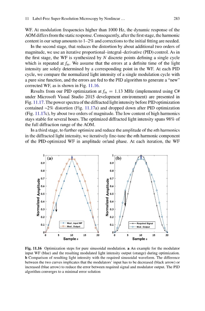
cycle, we compare the normalized light intensity of a single modulation cycle with
a pure sine function, and the errors are fed to the PID algorithm to generate a “new”
corrected WF, as is shown in Fig. 11.16.
Results from our PID optimization at f m = 1.13 MHz (implemented using C#
under Microsoft Visual Studio 2015 development environment) are presented in
Fig. 11.17. The power spectra of the diffracted light intensity before PID optimization
contained ~2% distortion (Fig. 11.17a) and dropped down after PID optimization
(Fig. 11.17c), by about two orders of magnitude. The low content of high harmonics
stays stable for several hours. The optimized diffracted light intensity spans 98% of
the full diffraction range of the AOM.
In a third stage, to further optimize and reduce the amplitude of the nth harmonics
in the diffracted light intensity, we iteratively fine-tune the nth harmonic component
of the PID-optimized WF in amplitude or/and phase. At each iteration, the WF
0
5
10
15
20
Sample #
0
0.1
0.2
0.3
0.4
0.5
0.6
0.7
0.8
0.9
1
Normalized
Amplitude
Mod . input WF
Mod . Output
0
5
10
15
20
Sample #
0
0.1
0.2
0.3
0.4
0.5
0.6
0.7
0.8
0.9
1
Normalized
Amplitude
Required Signal
Mod . Output
(a)
(b)
Fig. 11.16 Optimization steps for pure sinusoidal modulation. a An example for the modulator
input WF (blue) and the resulting modulated light intensity output (orange) during optimization.
b Comparison of resulting light intensity with the required sinusoidal waveform. The difference
between the two curves implicates that the modulators’ input has to be decreased (black arrow) or
increased (blue arrow) to reduce the error between required signal and modulator output. The PID
algorithm converges to a minimal error solution
283
WF. At modulation frequencies higher than 1000 Hz, the dynamic response of the
AOM differs from the static response. Consequently, after the first stage, the harmonic
content in our setup amounts to 1–2% and corrections to the initial fitting are needed.
In the second stage, that reduces the distortion by about additional two orders of
magnitude, we use an iterative proportional–integral–derivative (PID) control. As in
the first stage, the WF is synthesized by N discrete points defining a single cycle
which is repeated at f m . We assume that the errors at a definite time of the light
intensity are solely determined by a corresponding point in the WF. At each PID
cycle, we compare the normalized light intensity of a single modulation cycle with
a pure sine function, and the errors are fed to the PID algorithm to generate a “new”
corrected WF, as is shown in Fig. 11.16.
Results from our PID optimization at f m = 1.13 MHz (implemented using C#
under Microsoft Visual Studio 2015 development environment) are presented in
Fig. 11.17. The power spectra of the diffracted light intensity before PID optimization
contained ~2% distortion (Fig. 11.17a) and dropped down after PID optimization
(Fig. 11.17c), by about two orders of magnitude. The low content of high harmonics
stays stable for several hours. The optimized diffracted light intensity spans 98% of
the full diffraction range of the AOM.
In a third stage, to further optimize and reduce the amplitude of the nth harmonics
in the diffracted light intensity, we iteratively fine-tune the nth harmonic component
of the PID-optimized WF in amplitude or/and phase. At each iteration, the WF
0
5
10
15
20
Sample #
0
0.1
0.2
0.3
0.4
0.5
0.6
0.7
0.8
0.9
1
Normalized
Amplitude
Mod . input WF
Mod . Output
0
5
10
15
20
Sample #
0
0.1
0.2
0.3
0.4
0.5
0.6
0.7
0.8
0.9
1
Normalized
Amplitude
Required Signal
Mod . Output
(a)
(b)
Fig. 11.16 Optimization steps for pure sinusoidal modulation. a An example for the modulator
input WF (blue) and the resulting modulated light intensity output (orange) during optimization.
b Comparison of resulting light intensity with the required sinusoidal waveform. The difference
between the two curves implicates that the modulators’ input has to be decreased (black arrow) or
increased (blue arrow) to reduce the error between required signal and modulator output. The PID
algorithm converges to a minimal error solution