

272
O. Tzang et al.
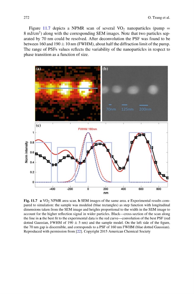
Figure 11.7 depicts a NPMR scan of several VO 2 nanoparticles (pump =
8 mJ/cm
2 ) along with the corresponding SEM images. Note that two particles separated by 70 nm could be resolved. After deconvolution the PSF was found to be
between 160 and 190 ± 10 nm (FWHM), about half the diffraction limit of the pump.
The range of PSFs values reflects the variability of the nanoparticles in respect to
phase transition as a function of size.
Fig. 11.7 a VO 2 NPMR area scan. b SEM images of the same area. c Experimental results compared to simulation: the sample was modeled (blue rectangles) as step function with longitudinal
dimensions taken from the SEM image and heights proportional to the width in the SEM image to
account for the higher reflection signal in wider particles. Black—cross-section of the scan along
the line in a the best fit to the experimental data is the red curve—convolution of the best PSF (red
dotted Gaussian, FWHM of 190 ± 5 nm) and the sample model. On the left side of the figure,
the 70 nm gap is discernible, and corresponds to a PSF of 160 nm FWHM (blue dotted Gaussian).
Reproduced with permission from [22]. Copyright 2015 American Chemical Society
O. Tzang et al.
Figure 11.7 depicts a NPMR scan of several VO 2 nanoparticles (pump =
8 mJ/cm
2 ) along with the corresponding SEM images. Note that two particles separated by 70 nm could be resolved. After deconvolution the PSF was found to be
between 160 and 190 ± 10 nm (FWHM), about half the diffraction limit of the pump.
The range of PSFs values reflects the variability of the nanoparticles in respect to
phase transition as a function of size.
Fig. 11.7 a VO 2 NPMR area scan. b SEM images of the same area. c Experimental results compared to simulation: the sample was modeled (blue rectangles) as step function with longitudinal
dimensions taken from the SEM image and heights proportional to the width in the SEM image to
account for the higher reflection signal in wider particles. Black—cross-section of the scan along
the line in a the best fit to the experimental data is the red curve—convolution of the best PSF (red
dotted Gaussian, FWHM of 190 ± 5 nm) and the sample model. On the left side of the figure,
the 70 nm gap is discernible, and corresponds to a PSF of 160 nm FWHM (blue dotted Gaussian).
Reproduced with permission from [22]. Copyright 2015 American Chemical Society